Кластер
Итак , вам нужен кластер
Что это такое кластер и для чего он нужен?
По-сути , это супер-компьютер ,который может построить каждый.
Cluster - это компьютер с параллельной архитектурой ,
построенный из множества компонентов.
Этот подход основан на использовании персональных компьютеров.
Скорость вычислений , размер памяти , доступное дисковое пространство в сумме дают выигрыш.
Фактически , если взять первые пять супер-компьютеров из списка "Top500" ,
они представляют из себя кластеры.
A Beowulf cluster is a form of parallel computer, which is nothing more than a computer that uses more than one processor. There are many different kinds of parallel computer, distinguished by the kinds of processors they use and the way in which those processors exchange data. A Beowulf cluster takes advantage of two commodity components: fast CPUs designed primarily for the personal computer market and networks designed to connect personal computers together (in what is called a local area network or LAN). Because these are commodity components, their cost is relatively low. As we will see later in this chapter, there are some performance consequences, and Beowulf clusters are not suitable for all problems. However, for the many problems for which they do work well, Beowulf clusters provide an effective and low-cost solution for delivering enormous computational power to applications and are now used virtually everywhere. This raises the following question: If Beowulf clusters are so great, why didn't they appear earlier?
Many early efforts used clusters of smaller machines, typically workstations, as building blocks in creating low-cost parallel computers. In addition, many software projects developed the basic software for programming parallel machines. Some of these made their software available for all users, and emphasized portability of the code, making these tools easily portable to new machines. But the project that truly launched clusters was the Beowulf project at the NASA Goddard Space Flight center. In 1994, Thomas Sterling, Donald Becker, and others took an early version of the Linux operating system, developed Ethernet driver software for Linux, and installed PVM (a software package for programming parallel computers) on 16 100MHz Intel 80486-based PCs. This cluster used dual 10-Mbit Ethernet to provide improved bandwidth in communications between processors, but was otherwise very simple—and very low cost.
Why did the Beowulf project succeed? Part of the answer is that it was the right solution at the right time. PCs were beginning to become competent computational platforms (a 100MHz 80486 has a faster clock than the original Cray 1, a machine considered one of the most important early supercomputers). The explosion in the size of the PC market was reducing the cost of the hardware through economies of scale. Equally important, however, was a commitment by the Beowulf project to deliver a working solution, not just a research testbed. The Beowulf project worked hard to "dot the i's and cross the t's," addressing many of the real issues standing in the way of widespread adoption of cluster technology for commodity components. This was a critical contribution; making a cluster solid and reliable often requires solving new and even harder problems; it isn't just hacking. The contribution of the community to this effort, through contributions of software and general help to others building clusters, made Beowulf clustering exciting.
Since the early Beowulf clusters, the use of commodity-off-the-shelf (COTS) components for building clusters has mushroomed. Clusters are found everywhere, from schools to dorm rooms to the largest machine rooms. Large clusters are an increasing percentage of the Top500 list. You can still build your own cluster by buying individual components, but you can also buy a preassembled and tested cluster from many vendors, including both large and well-established computer companies and companies formed just to sell clusters.
This book will give you an understanding of what Beowulfs are, where they can be used (and where they can't), and how they work. To illustrate the issues, specific operations, such as installation of a software package are described. However, this book is not a cookbook; software and even hardware change too fast for that to be practical. The best use of this book is to read it for understanding; to build a cluster, then go out and find the most up-to-date information on the web about the hardware and software.
Each of the areas discussed in this book could have its own book. In fact, many do, including books in the same MIT Press series. What this book does is give you the basic background so that you can understand Beowulf Clusters. For those areas that are central to your interest in Beowulf computing, we recommend that you read the relevant books. Some of these are described in Appendix B. For the others, this book provides a solid background for understanding how to specify, build, program, and manage a Beowulf cluster.
We begin by defining what a cluster is and why a cluster can be a good computing platform. Since not all applications are appropriate for clusters, Section 1.3 introduces techniques for estimating the performance of an application on a cluster, with an illustration drawn from technical computing. With this background, the next two sections provide two different ways to read this book. Section 1.4 provides a procedural approach, from choosing which components will constitute the cluster to determining how applications can be tuned on the cluster. Section 1.5 provides a topical approach, such as how to program it, run jobs on it, or specify a cluster's components.
Chapter 2: Node Hardware
Highlights
Narayan Desai and Thomas Sterling
Few technologies in human civilization have experienced such a rate of growth as that of the digital computer and its culmination in the PC. Its low cost, ubiquity, and sometimes trivial application often obscure its complexity and precision as one of the most sophisticated products derived from science and engineering. In a single human lifetime over the fifty-year history of computer development, performance and memory capacity have grown by a factor of almost a million. Where once computers were reserved for the special environments of carefully structured machine rooms, now they are found in almost every office and home. A personal computer today outperforms the world's greatest supercomputers of two decades ago at less than one ten-thousandth the cost. It is the product of this extraordinary legacy that Beowulf harnesses to open new vistas in computation.
A Beowulf cluster is a network of nodes, with each node a low-cost personal computer. Its power and simplicity are derived from exploiting the capabilities of the mass-market systems that provide both the processing and the communication. This chapter explores the hardware elements related to computation and storage. The choice of node hardware, along with the choice of a system area network, will determine the basic performance properties of the Beowulf for its entire operational lifetime. Neither of these choices should be taken lightly; tremendous variation exists among instances of all components involved. This chapter discusses the components included in a cluster node, their function in a system, and their effects on node performance. Communication hardware is discussed in detail in Chapter 4. The purpose of a Beowulf cluster is to perform parallel computations. This is accomplished by running applications across a number of nodes simultaneously. These applications may perform in parallel; that is, they may need to coordinate during execution. On the other hand, they may be performing an embarrassingly parallel task, or a large group of serial tasks. One key factor in application performance in all cases is local node performance.
2.1 Node Hardware OverviewA cluster node is responsible for all activities and capabilities associated with executing an application program and supporting a sophisticated software environment. The process of application involves a large number of components. An application is actually executed on the main CPU. The CPU loads data from its cache and main memory into registers. All applications use peripherals, such as persistent storage or network transmission, for noncomputational tasks. All peripherals load data into or process data from main memory, where it can be accessed by the system CPU. Applications can be characterized in terms of these three basic operations:
-
Instruction execution: operating on data in registers, storing the results in term in registers. This operation is implemented entirely by the CPU.
-
Register loading: loading data from main memory or processor cache into processor registers to facilitate instruction execution. This operation involves the CPU, front-side bus, and system memory.
-
Peripheral usage: copying data across an I/O bus into or out of main memory to allow for a noncomputational task to occur. This operation involves the peripheral, the I/O bus, and the interface from the I/O bus into system memory, and system memory itself.
The system CPU is the main processor, on which most code is executed. A node may have more than one of these, operating in SMP (symmetric multiprocessing) mode. This processor will have some amount of cache. Cache is used for fast access to data in main memory. Cache is typically ten times faster than main memory, so it is advantageous to load data into cache before using it. Main memory is the location where running programs, including the operating system, store all data. It is not persistent; data that should survive beyond a reboot is copied to some persistent medium, such as a hard disk. An I/O bus connects main memory with all peripherals. The peripherals (disk controllers, network controllers, video cards, etc.) operate by manipulating data from main memory. For example, a disk write will occur by copying data across the I/O bus to the disk controller. The disk controller will then actually write the data to disk.
In detail, when an application is executed, it is loaded from disk or some other persistent storage into main memory. When execution actually begins, parts of the application are copied into processor cache. From here, the data is written into on-processor registers, where the processor can directly access it. When the processor is done with this data, it is copied back out to main memory. When the application is dependent on data from a peripheral (e.g., data read from hard disk, or data received on a network interface) loading data into registers becomes much more complex. For example, a kernel call will result in a disk controller's reading of data from hard disk into local storage on the controller. The controller will copy the data across the I/O bus to system main memory, from which it can be loaded into registers for the processor to operate on. Each of these steps is faster than the proceeding step; indeed, there are several orders of magnitude difference between the speeds of the first step and the last step. All applications can be characterized in terms of these basic three types of activities.
2.2 MicroprocessorA microprocessor (also referred to as the CPU or processor) is at the heart of any computer. It is the single component that implements instruction execution. Processors vary in a number of ways; we focus on the more important characteristics. The lowest-level binary encoding of the instructions and the actions they perform are dictated by the microprocessor instruction set architecture (ISA). The most common ISA used for cluster node CPU is IA32, or X86. This family of processors includes all generations of the Pentium processor and the Athlon family. A shared ISA doesn't imply an identical instruction set; newer processors have extra features that old processors do not. For example, SSE and SSE2 are numerical instruction sets that were added in Pentium III and Pentium 4 processors, respectively. The earliest clusters were composed of 486 processors, which implement this ISA.
A processor runs at a particular clock rate. That is, it can execute instructions at a particular frequency, measured in terms of megahertz or gigahertz. For example, a 2.4 GHz processor can execute a rate of 2.4 billion instructions per second. Note that a processor's clock rate is not a direct measure of performance. Frequently, processors with different clock rates can perform equivalently for some tasks; likewise, two processors with the same clock rate can perform quite differently for some tasks. Current clock rates range from 1 GHz to slightly over 3 GHz.
Any processor has a theoretical peak speed. Theoretical peak is the maximum rate of instruction execution a processor can achieve. This is determined by the clock rate, ISA, and components included in the processor itself. This rate is measured in floating-point operations per second, or flops. A current generation processor will have a theoretical peak of 3–5 gigaflops. As one might guess from the name, theoretical peak is just that, theoretical. A processor rarely, if ever, runs at that rate while executing a real user application.
Both the instructions and the data upon which they act are stored in and loaded from the node's random access memory (RAM). The speed of a processor is often measured in megahertz, indicating that its clock ticks so many million times per second. RAM runs at a much slower clock rate, usually measured in hundreds of megahertz. Thus, the processor often waits for memory, and the overall rate at which programs run is usually governed as much by the memory system as by the processor's clock speed.
The slow rate at which data can be copied from RAM is mitigated by a processor's cache. The cache is a small amount of fast memory usually co-located on the CPU. When data is copied from main memory, it is also stored in cache. If the same data is accessed again, it can be read from cache. This is highly advantageous: applications can be optimized to access memory in patterns that take the best possible advantage of cache speed. The quicker access to memory in cache leads to better processor utilization; the processor spends less time waiting for data from memory. Processor caches vary in size from kilobytes on some processors to upwards of four to eight megabytes on processors specified to provide good floating point performance. Obviously, the larger the cache is, the easier it is to reuse entries stored in it.
2.2.1 IA32
IA32 is the most common ISA used in clusters today, and for the foreseeable future. This is caused by the enormous economies of scale at work. Processors implementing this ISA are used in the majority of desktop PCs sold. IA32 is a 32-bit instruction set. It is treated as a binary compatibility specification. Multiple processors, implemented in vastly different ways, all implement the same instruction set to allow for application portability. The three most common processors used in clusters today are the Pentium III and 4 processors, manufactured by Intel, and AMD's Athlon processor. Recent additions to the IA32 ISA include SSE and its successor SSE2. (Streaming SIMD Extensions) SSE and SSE2 are instruction set extensions that define instructions that can be performed in parallel on multiple data elements; these are not necessarily implemented in all instances of IA32 processors. These features can yield substantially improved performance, so care should be taken when choosing the processor for a new system. Hyperthreading is another feature recently added to the IA32 ISA. It allows multiple threads of execution per physical CPU. This feature typically impacts application performance negatively and can be disabled, so it really isn't a decision point when choosing a CPU, as SSE and SSE2 are.
Pentium 4. The Pentium 4 implements the IA32 instruction set but uses an internal architecture that diverges substantially from the old P6 architecture. The internal architecture is geared for high clock speeds; it produces less computing power per clock cycle but is capable of extremely high frequencies. This architecture is also the only IA32 processor family that implements the SSE2 instruction set, providing a substantial performance benefit for some applications. This is also the only architecture that implements hyperthreading, but (as was mentioned previously) this feature is not terribly important for computational applications typically run on clusters.
Pentium III. The Pentium III is based on the older Pentium Pro architecture. It is a minor upgrade from the Pentium II; it includes SSE for three-dimensional instructions and has moved the L2 cache onto the chip, making it synchronized with the processor's clock. The Pentium III can be used within an SMP node with two processors; a more expensive variant, the Pentium III Xeon, can be used in four-processor SMP nodes.
Athlon. The AMD Athlon platform is similar to the Pentium III in its processor architecture but similar to the Compaq Alpha in its bus architecture. It has two large 64 KByte L1 caches and a 256 KByte L2 cache that run at the processor's clock speed. The performance is a little better than that of the Pentium III and Pentium 4 in general at similar clock rates, but either can be faster depending on the application. The Athlon supports dual-processor SMP nodes. Newer Athlon processors support SSE, but not SSE2.
2.2.2 Other Processor Types
HP Alpha 21264. The Compaq (now HP and originally DEC) Alpha processor is a true 64-bit architecture. For many years, the Alpha held the lead in many benchmarks, including the SPEC benchmarks, and was used in many of the fastest supercomputers, including the Cray T3D and T3E, as well as the Compaq SC family. Alpha are still popular with some users, but since the Alpha processor line is no longer being developed and the current Alpha processor will be the last, Alphas are rarely chosen for new systems. However, a few large clusters make use of Alphas, including the ASCI Q system at Los Alamos National Laboratory; ASCI Q is one of the fastest systems in the world, according to the Top500 list.
The Alpha uses a Reduced Instruction Set Computer (RISC) architecture, distinguishing it from Intel's Pentium processors. RISC designs, which have dominated the workstation market of the past decade, eschew complex instructions and addressing modes, resulting in simpler processors running at higher clock rates, but executing somewhat more instructions to complete the same task.
PowerPC G5. The IBM PowerPC is an processor architecture used in products from IBM and from Apple. The newest processor is the G5, a sophisticated 64-bit processor capable of running at speeds of up to 2GHz. Other features include a 1GHz frontside bus and multiple functional units, allowing the G5 to perform multiple operations in each clock cycle. Apple sells Macs with the G5 processor, and a number of groups have built clusters using Macs, running Mac OS X (a Unix-like operating system).
IA64. The IA64 is Intel's first 64-bit architecture. This is an all-new design, with a new instruction set, new cache design, and new floating-point processor design. With clock rates approaching 1 GHz and multiway floating-point instruction issue, Itanium should be the first implementation to provide between 1 and 2 Gflops peak performance. The first systems with the Itanium processor were released in the middle of 2001 and have delivered impressive results. For example, the HP Server rx4610, using a single 800 MHz Itanium, delivered a SPECfp2000 of 701, comparable to recent Alpha-based systems. More recent results with a 1.5 GHz Itanium 2 in an HP rx2600 server gave a SPECfp2000 of 2119. The IA64 architecture does, however, require significant help from the compiler to exploit what Intel calls EPIC (explicitly parallel instruction computing).
Opteron. Another 64-bit architecture is AMD's Opteron. Unlike the Intel IA64 architecture, the Opteron supports both the IA32 instruction set as well as a new 64-bit extension, allowing users to continue to use their existing 32-bit applications while taking advantage of a 64-bit instruction set for applications that require easy access to more than 4 GB of memory. The Opteron includes an integrated DDR memory controller and a high-performance interconnect called "HyperTransport" that provides up to 6.4 GB/sec bandwidth per link; each Opteron may have three HyperTransport links. Early Opterons have delivered a SPECfp2000 of 1154. The AMD Opteron is used in the Cray "Red Storm," that will use over 10,000 processors and have a peak performance of over 40 Teraflops.
2.3 MemoryA system's random access memory (RAM, or memory) is a temporary storage location used to store instructions and data. Instructions are the actual operations a processor executes. The data comes from a variety of sources. It may be data supplied by some peripheral, such as a hard disk or network controller. It may be intermediary results generated during program execution. Instructions and data are both required for the processor to compute a meaningful result. Hence, the processor constantly is issuing commands to load or store data from memory across the memory bus. Memory buses operate at rates between 100 MHz and 800 MHz. This bus is also referred to as the front side bus, or FSB.
Because of the constant usage of system RAM and the large gap between processor clock rate and memory bus rate, the memory bus is one of the largest impediments to achieving theoretical peak. Memory bus performance is measured in terms of two characteristics. The first is peak memory bandwidth, the burst rate that data can be copied between the DRAM chips in main memory and the CPU. The FSB must be fast enough to support this high burst rate. In the case of some proprietary systems, memory accesses are pipelined to improve aggregate memory bandwidth. In this case, data is bursted from multiple groups of DRAM chips. However, this technique is not used in PC systems. The second characteristic is memory latency, the amount of time it takes to move data between RAM and the CPU. RAM bandwidth ranges from one to four gigabytes per second. RAM latency has fallen to under 6 nanoseconds.
Except for very carefully designed applications, a program's entire dataset must reside in RAM. The alternative is to use disk storage either explicitly (out-of-core calculations) or implicitly (virtual memory swapping), but this usually entails a severe performance penalty. Thus, the size of a node's memory is important in parameter in system design. It determines the size of problem that can practically be run on the node. Engineering and scientific applications often obey a rule of thumb that says that for every floating-point operation per second, one byte of RAM is necessary. This is a gross approximation at best, and actual requirements can vary by many orders of magnitude, but it provides some guidance; for example, a 1 GHz processor capable of sustaining 200 Mflops should be equipped with approximately 200 MBytes of RAM.
Two main types of RAM are used in current commodity systems. SDRAM has been in use for several years. RDRAM is a newer standard used only in Pentium 4-based systems. RDRAM tends to be faster and more expensive.
2.4 I/O ChannelsI/O channels are buses that connect peripherals with main memory. These peripherals will range from disk and network controllers to video controllers, and USB and firewire. Machines will have several of these buses, each connected by a bridge (also referred to as the PCI chipset) into main memory. Because I/O is one of the most common tasks on computers, this subsystem is an integral part of any system.
2.4.1 PCI and PCI-X
The most common I/O channel in commodity hardware is the PCI bus. Every machine sold today has at least one; many have multiples of these buses. Many flavors of PCI exist; these buses have been included in commodity hardware since 1994. Earlier versions of the PCI bus were 32-bit, 33 MHz buses. The theoretical maximum rate of data transmission on these buses is 132 MB/s. Good implementations of the PCI chipset are able to provide nearly this rate; maximum observed bus rates greater than 125 MB/s are not uncommon.
Newer revisions of PCI buses are 64-bit buses, running at 66 MHz or higher. These buses have become quite common over the last three to four years. The theoretical maximum rate for these is upwards of 500 MB/s. Good implementations of this PCI chipset provide between 400 and 500 MB/s of read and write bandwidth. Good PCI-X implementations, running at 133 MHz, provide upwards on 900 MB/s of read and write bandwidth.
2.4.2 AGP
AGP is a port used for high-speed graphics adapters. It is connected closely with main memory, providing better peak bandwidth than that offered by PCI or PCI-X. AGP devices are able to directly use data out of main memory. AGP is not a bus, like PCI. It is only able to support one device, and systems only have one port. AGP 2.0 provided a peak bandwidth over 1 GB/s to main memory. The successor to this, AGP 3.0, provides upwards of 2.1 GB/s to main memory.
2.4.3 Legacy Buses
Older machines will also have other buses. The ISA bus is an 8 or 16-bit bus, commonly used in older machines. Vesa local bus is a 24-bit bus, common in some generations of 486 machines. EISA is an extension to ISA that was common in older servers. All of these buses should be avoided if possible: They are slow, and peripheral choice is non-existent.
2.5 MotherboardThe motherboard is a printed circuit board that contains most of the active electronic components of the PC node and their interconnection. The motherboard provides the logical and physical infrastructure for integrating the subsystems of a cluster node and determines the set of components that may be used. The motherboard defines the functionality of the node, the range of performance that can be exploited, the maximum capacities of its storage, and the number of subsystems that can be interconnected. With the exception of the microprocessor itself, the selection of the motherboard is the most important decision in determining the qualities of the PC node to be used as the building block of the system. It is certainly the most obvious piece of a node other than the case or packaging in which it is enclosed.
The motherboard integrates all of the electronics of the node in a robust and configurable package. Sockets and connectors on the motherboard include the following:
-
Microprocessor(s)
-
Memory
-
Peripheral controllers on the PCI-X bus
-
AGP port
-
Floppy disk cables
-
ATA or SCSI cables for hard disk and CD-ROM
-
Power
-
Front panel LEDs, speakers, switches, and so forth.
-
External I/O for mouse, keyboard, joystick, serial line, sound, USB, and so forth.
Other chips on the motherboard provide
-
the system bus that links the processor(s) to memory,
-
the interface between the peripheral buses and the system bus, and
-
programmable read-only memory (PROM) containing the BIOS software.
As the preceding lists show, motherboards are an amalgamation of all of the buses and many peripherals in a cluster node. The memory bus is contained within the motherboard. All I/O buses a system supports are also included here. As data movement is the most serious impediment to achieving peak processor performance, the motherboard is one of the single most important components in a system.
We note that the motherboard restricts as well as enables functionality. In selecting a motherboard as the basis for a cluster node, one should consider several requirements including
2.5.1 Chipsets
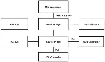
Chipsets are a combination of all of the logic on a motherboard. Typically included are the memory bus, PCI, PCI-X and AGP bridges. In many cases, integrated peripherals are also part of the chipset. This may include disk controllers and USB controllers. Because the chipset combines all of these components, performance properties of single components are often attributed to the chipset itself.
The chipset is split into two logical portions. The north bridge connects the front side bus, which connects the processor, the memory bus, and AGP. AGP is located on the north bridge so as to have special access to main memory. The south bridge contains I/O bus bridges and any integrated peripherals that may be included, like disk and USB controllers. This provides controllers for all of the simple devices mentioned later in the peripherals section.
2.5.2 BIOS
The BIOS is the software that initializes all system hardware into a state such that the operating system can boot. BIOSes are not universal; that is, the BIOS included with a motherboard is specifically tailored to that motherboard. The BIOS is the first software that runs after the system is powered up. The BIOS will start by running a power on self test (POST) that includes this ubiquitous memory test. POST also checks other major systems. The BIOS runs initialization code present on peripherals, including controller-specific code that initializes SCSI or IDE buses. Once these steps are completed, the BIOS locates a drive to boot from, and does so.
PXE (Pre-execution environment) is a system by which nodes can boot based on a network-provided configuration and boot image. The system is implemented as a combination of two common network services. First, a node will DHCP for an address. The DHCP server will return an offer and lease with extra PXE data. This extra data contains an IP address of a tftp server, a boot image filename (that is served from the server), and an extra configuration string that is passed to the boot image. Most new machines support this, and accordingly many cluster management software systems use this feature for installations. This feature is implemented by the BIOS in motherboards with integrated ethernet controllers, and in the on-card device initialization code on add-on ethernet controllers.
LinuxBIOS is a BIOS implementation based on the Linux kernel. It can perform all important tasks needed for an operating system to boot. These tasks are largely the same as proprietary BIOSes, but some of these steps have been streamlined in such a way that all operating systems do not function properly when booted from LinuxBIOS. At this point, Linux and Windows 2000 are supported. Work is under way to supply all BIOS features necessary to run other operating systems as well. This approach offers several benefits. Since source code is available for LinuxBIOS, the potential exists for users to fix BIOS bugs. LinuxBIOS is also performs far better than proprietary BIOSes in terms of boot time. This reduction has yielded boot times under five seconds. This speed is far better than times in the ten to ninety second range seen with proprietary BIOSes. This performance increase doesn't affect user applications, as most user applications don't require node reboots.
2.6 Persistent StorageWith the exception of BIOS code and configuration, all data stored in memory is lost when power cycles occur. In order to store data persistently, non-volatile storage medium is required. Specifically, data from a system's main memory is usually stored on some sort of disk when applications are not using it. It is then loaded when the application needs it again.
2.6.1 Local Hard Disks
Most clusters have a hard disk on each node for some storage. This is usually used in addition to a central data storage facility. Hard disks are magnetic storage media that interface with some sort of storage bus. A hard drive will contain several platters. Data is read off of these platters as they rotate. Logic in the drive optimizes read and write requests based on the geometry of the disk to provide better collective performance. This logic also contains memory cache, which is used to prevent the need for multiple reads of the same data.
Disks also have an interface to any of a number of disk buses. The three most common buses currently in use for commodity disks are IDE (or EIDE or ATA), SCSI, and Serial ATA. IDE disks are the most common. Controllers are integrated into nearly every motherboard sold today. These controllers support two devices per bus and typically include two buses, for a total of four devices. The fastest of these buses, UDMA133 (Ultra DMA 133), run at rates up to 133 MB/s. IDE devices are typically implemented with less logic on each drive, leading to higher host CPU utilization during I/O when compared with SCSI.
SCSI disks are typically used in servers. Everything but the bus interface logic is nearly identical in many disks, regardless of disk interface bus. Many vendors sell multiple versions of many of their drives, one for each bus type. That said, the major difference between IDE and SCSI disks is the obvious one: the data bus. SCSI buses support many more devices and run at higher speeds. Current SCSI buses support up to fifteen devices and the controller, which functions as a SCSI device as well. Current-generation SCSI buses operate at rates up to 320 MB/s. This higher data rate is needed because of the larger quantities of devices sharing a single bus. The largest differentiating characteristic between IDE and SCSI disks is the cost at this point; SCSI disks are more expensive.
Serial ATA, or SATA, is the newest commodity disk standard. New, high-end motherboards are beginning to incorporate controllers. Nominally, Serial ATA is similar to IDE/ATA. Those older standards are now referred to collectively as Parallel ATA, or PATA. SATA is poised to take over the market segment of PATA; drives are not quite price competitive at this time, but their prices are close enough that in the next few months, they should drop to PATA levels. Serial ATA, as the name suggests, is a serial bus as opposed to the parallel buses used PATA and SCSI. Hence, the cables attached to drives are smaller and run faster: current SATA connections function at 150 MB/s. Because SATA buses are only used by two devices, the aggregate data rate doesn't need to be as high as those on parallel buses to perform comparably. Because of the serial nature of SATA, bus speeds will increase rapidly, when compared with parallel buses like PATA and SCSI. SATA is natively hot-pluggable, and its cables are far smaller than the ribbon cables used by PATA and SCSI. The increased speed of SATA buses doesn't provide a real benefit at this point; most drives don't function at speeds high enough to congest a high-speed PATA controller.
The same basic disk technology is used in disks using any of the three previously mentioned buses. Hence, the basic measures of performance are the same as well. The platters in disks spin at a variety of rates. The faster the platters spin, the faster data can be read off of the disk, and data on the far end of the platters will become available sooner. Rotational speeds range from 5,400 RPM to 15,000 RPM. The faster the platters rotate, the lower latency and higher bandwidth are. The other main indicator of performance of a disk is the amount of cache included in the on-disk controller. As was mentioned previously, this cache is used to avoid disk reads when particular blocks on the disk are requested multiple times.
2.6.2 RAID
RAID, or Redundant Array of Inexpensive Disks, is a mechanism by which the performance and storage properties of individual disks can be aggregated. Aggregation may be done for a variety of reasons. Simplification of disk layout is the most common. Basically, the group of disks appear to be a single larger disk. This approach is commonly used when disks are in use that are not as large as the data that will be stored. Performance is another common reason. Multiple disks will perform better than single disks. The last reason RAID is used is to guard against hardware failure. When multiple disks are used in a RAID set, data can be stored in multiple places. This approach allows the system to continue functioning with no loss of data after disk faults. These solutions can be implemented in software, usually as an operating system driver, or in hardware, typically consisting of disk controllers, a processor that handles RAID functions, and a host connection. Hardware solutions tend to be more expensive but also tend to perform better without impacting host CPU utilization. Software solutions typically allow more flexibility, but the computational overhead of some RAID levels can consume large amounts of computational resources.
A variety of allocation schemes are used in RAID systems. With RAID0, or striping, data is striped across multiple disks. The result of this striping is a logical storage device that has the capacity of each of the disks times the number of disks present in the array. This array performs differently from a single larger disk. Reads are accelerated; each byte of data can be read from multiple locations, so interleaving reads between disks can double read performance. Write performance is similarly accelerated, as actually disk write performance is improved compared with that of a single disk.
With RAID1, or mirroring, complete copies of the data are stored in multiple locations. The capacity of one of these RAID sets will be half of its raw capacity. In this configuration, reads are accelerated in a similar manner to RAID0, but writes are slowed, as new data needs to be transmitted multiple times, to both parts of the mirror.
The third common RAID level is RAID5. It works similarly to RAID0, in that data is spread across multiple disks, with one addition. One disk is used to store parity information. This means for any block of data stored across the N-1 drives in an array, a parity checksum is computed and stored on the last disk. This allows the array to continue functioning in case of drive failure, as the parity checksum can be used in the place of a block off of any one of the data disks. Read performance on RAID5 volumes tend to be quite good, but write performance lags behind mirrors because of the overhead of checksum computation. This overhead can cause performance problems when using software RAID.
RAID is typically used on storage nodes in clusters. The reasons for this are the performance and capacity differences when compared to standalone disks. These disk I/O characteristics are not of prime import on compute nodes, so RAID is not typically configured there.
2.6.3 Nonlocal Storage
Nonlocal storage is used in similar ways to local storage. Data that needs to survive system power cycles is stored there. The physical medium on which data is stored is similar, if not identical, to the hard disk technology described in the preceding sections: the difference lies in the data transport layer. In the case of nonlocal storage, the storage device bus traffic is transmitted across a network to a central depot of storage. This network may or may not be dedicated to storage; standards exist for protocols of both types.
ISCSI is a protocol that encapsulates SCSI commands and data inside IP packets. These are typically transmitted over ethernet. It allows a single network to be used for disk I/O and regular network traffic, however, this can form a serious performance bottleneck. Fiberchannel is similar to ISCSI in character, but uses a dedicated network and data protocol.
Network filesystems are most common in clusters. Examples of this include NFS and PVFS. (PVFS is discussed in detail in Section 19) Network filesystems transmit persistent data across a network, but differ from the previous two storage types in the nature of the data being transmitted. Network filesystems transmit data with filesystem semantics across the network; the previous two protocols transmit block-based data.
3.2 The Linux Kernel
As mentioned earlier, for the Beowulf user, a smaller, faster, and leaner kernel is a better kernel. This section describes the important features of the Linux kernel for Beowulf users and shows how a little knowledge about the Linux kernel can make the cluster run faster and more smoothly.
What exactly does the kernel do? Its first responsibility is to be an interface to the hardware and provide a basic environment for processes and memory management. When user code opens a file, requests 30 megabytes of memory for user data, or sends a TCP/IP message, the kernel does the resource management. If the Linux server is a firewall, special kernel code can be used to filter network traffic. In general, there are no additives to the Linux kernel to make it better for scientific clusters—usually, making the kernel smaller and tighter is the goal. However, sometimes a virtual memory management algorithm can be twiddled to improve cache locality, since the memory access patterns of scientific applications are often much different from the patterns common Web servers and desktop workstations, the applications for which Linux kernel parameters and algorithms are generally tuned. Likewise, occasionally someone creates a TCP/IP patch that makes message passing for Linux clusters work a little better. Before going that deep into Linux kernel tuning, however, the kernel must first simply be compiled.
3.2.1 Compiling a Kernel
Almost all Linux distributions ship with a kernel build environment that is ready for action. The transcript below shows how you can learn a bit about the kernel running on the system.
The '/proc' file system is not really a file system in the traditional meaning. It is not used to store files on the disk or some other secondary storage; rather, it is a pseudo-file system that is used as an interface to kernel data structures—a window into the running kernel. Linus likes the file system metaphor for gaining access to the heart of the kernel. Therefore, the '/proc' file system does not really have disk filenames but the names of parts of the system that can be accessed. In the example above, we read from the handle '/proc/version' using the Unix cat command. Notice that the file size is meaningless, since it is not really a file with bytes on a disk but a way to ask the kernel "What version are you currently running?" We can see the version of the kernel and some information about how it was built.
The source code for the kernel is often kept in '/usr/src'. Usually, a symbolic link from '/usr/src/linux' points to the kernel currently being built. Generally, if you want to download a different kernel and recompile it, it is put in '/usr/src', and the symlink '/usr/src/linux' is changed to point to the new directory while you work on compiling the kernel. If there is no kernel source in '/usr/src/linux', you probably did not select "kernel source" when you installed the system for the first time, so in an effort to save space, the source code was not installed on the machine. The remedy is to get the software from the company's Web site or the original installation CD-ROM.
The kernel source code often looks something like the following:
If your Linux distribution has provided the kernel source in its friendliest form, you can recompile the kernel, as it currently is configured, simply by typing
The server will then spend anywhere from a few minutes to twenty or more minutes depending on the speed of the server and the size of the kernel. When it is finished, you will have a kernel.
3.2.2 Loadable Kernel Modules
For most kernels shipped with Linux distributions, the kernel is built to be modular. Linux has a special interface for loadable kernel modules, which provides a convenient way to extend the functionality of the kernel in a dynamic way, without retaining the code in memory all the time, and without requiring the kernel be recompiled every time a new or updated module arrives. Modules are most often used for device drivers, file systems, and special kernel features. For example, Linux can read and write MSDOS file systems. However, that functionality is usually not required at all times. Most often, it is required when reading or writing from an MSDOS floppy disk. The Linux kernel can dynamically load the MSDOS file system kernel module when it detects a request to mount an MSDOS file system. The resident size of the kernel remains small until it needs to dynamically add more functionality. By moving as many features out of the kernel core and into dynamically loadable modules, the legendary stability of Linux compared with legacy operating systems is achieved.
Linux distributions, in an attempt to support as many different hardware configurations and uses as possible, ship with as many precompiled kernel modules as possible. It is not uncommon to receive five hundred or more precompiled kernel modules with the distribution. In the example above, the core kernel was recompiled. This does not automatically recompile the dynamically loadable modules.
3.2.3 The Beowulf Kernel Diet
It is beyond the scope of this book to delve into the inner workings of the Linux kernel. However, for the Beowulf builder, slimming down the kernel into an even leaner and smaller image can be beneficial and, with a little help, is not too difficult.
In the example above, the kernel was simply recompiled, not configured. In order to slim down the kernel, the configuration step is required. There are several interfaces to configuring the kernel. The 'README' file in the kernel source outlines the steps required to configure and compile a kernel. Most people like the graphic interface and use make xconfig to edit the kernel configuration for the next compilation.
Removing and Optimizing
The first rule is to start slow and read the documentation. Plenty of documentation is available on the Internet that discusses the Linux kernel and all of the modules. However, probably the best advice is to start slow and simply remove a couple unneeded features, recompile, install the kernel, and try it. Since each kernel version can have different configuration options and module names, it is not possible simply to provide the Beowulf user a list of kernel configuration options in this book. Some basic principles can be outlined, however.
-
Think compute server: Most compute servers don't need support for amateur radio networking. Nor do most compute servers need sound support, unless of course your Beowulf will be used to provide a new type of parallel sonification. The list for what is really needed for a compute server is actually quite small. IrDA (infrared), quality of service, ISDN, ARCnet, Appletalk, Token ring, WAN, AX.25, USB support, mouse support, joysticks, and telephony are probably all useless for a Beowulf.
-
Optimize for your CPU: By default, many distributions ship their kernels compiled for the first-generation Pentium CPUs, so they will work on the widest range of machines. For your high-performance Beowulf, however, compiling the kernel to use the most advanced CPU instruction set available for your CPU can be an important optimization.
-
Optimize for the number of processors: If the target server has only one CPU, don't compile a symmetric multiprocessing kernel, because this adds unneeded locking overhead to the kernel.
-
Remove firewall or denial-of-service protections: Since Linux is usually optimized for Web serving or the desktop, kernel features to prevent or reduce the severity of denial-of-services attacks are often compiled into the kernel. Unfortunately, an extremely intense parallel program that is messaging bound can flood the interface with traffic, often resembling a denial-of-service attack. Indeed, some people have said that many a physicist's MPI program is actually a denial-of-service attack on the Beowulf cluster. Removing the special checks and detection algorithms can make the Beowulf more vulnerable, but the hardware is generally purchased with the intent to provide the most compute cycles per dollar possible, and putting it behind a firewall is relatively easy compared with securing and hampering every node's computation to perform some additional security checks. Section 5.6.2 discusses the use of firewalls with Beowulf clusters in more detail.
Other Considerations
Many Beowulf users slim down their kernel and even remove loadable module support. Since most hardware for a Beowulf is known, and scientific applications are very unlikely to require dynamic modules be loaded and unloaded while they are running, many administrators simply compile the required kernel code into the core. Particularly careful selection of kernel features can trim the kernel from a 1.5-megabyte compressed file with 10 megabytes of possible loadable modules to a 600-kilobyte compressed kernel image with no loadable modules. Some of the kernel features that should be considered for Beowulfs include the following:
-
NFS: While NFS does not scale to hundreds of node, it is very convenient for small clusters.
-
Serial console: Rather than using KVM (Keyboard, Video, Mouse) switches or plugging a VGA (video graphics array) cable directly into a node, it is often very convenient to use a serial concentrator to aggregate 32 serial consoles into one device that the system administrator can control.
-
Kernel IP configuration: This lets the kernel get its IP address from BOOTP or DHCP, often convenient for initial deployment of servers.
-
NFS root: Diskless booting is an important configuration for some Beowulfs. NFS root permits the node to mount the basic distribution files such as '/etc/passwd' from an NFS server.
-
Special high-performance network drivers: Often, an extreme performance Beowulf will use high-speed networking, such as Gigabit Ethernet or Myrinet. Naturally, those specialized drivers as well as the more common 100BT Ethernet driver can be compiled into the kernel.
-
A file system: Later in this chapter a more thorough discussion of file systems for Linux will be presented. It is important the kernel is compiled to support the file system chosen for the compute nodes
Network Booting
Because of the flexibility of Linux, many options are available to the cluster builder. While certainly most clusters are built using a local hard drive for booting the operating system, it is certainly not required. Network booting permits the kernel to be loaded from a network-attached server. Generally, a specialized network adapters or system BIOS is required. Until recently, there were no good standards in place for networking booting commodity hardware. Now, however, most companies are offering network boot-capable machines in their high-end servers. The most common standard is the Intel PXE 2.0 net booting mechanism. On such machines, the firmware boot code will request a network address and kernel from a network attached server, and then receive the kernel using TFTP (Trivial File Transfer Protocol). Unfortunately, the protocol is not very scalable, and attempting to boot more than a dozen or so nodes simultaneously will yield very poor results. Large Beowulfs attempting to use network boot protocols must carefully consider the number of simultaneously booting nodes or provide multiple TFTP servers and separate Ethernet collision domains. For a Linux cluster, performing a network boot and then mounting the local hard drive for the remainder of the operating system does not seem advantageous; it probably would have been much simpler to store the kernel on hard drive. However, network booting can be important for some clusters if it is used in conjunction with diskless nodes.
3.2.4 Diskless Operation
Some applications and environments can work quite well without the cost or management overhead of a hard drive. For example, in secure or classified computing environments, secondary storage can require special, labor-intensive procedures. In some environments, operating system kernels and distributions may need to be switched frequently, or even between runs of an application program. Reinstalling the operating system on each compute node to switch over the system is generally difficult, as would maintaining multiple hard disk partitions with different operating systems or configurations. In such cases, building the Beowulf without the operating system on the local hard drive, if it even exists, can be a good solution. Diskless operation also has the added benefit of making it possible to maintain only one operating system image, rather than having to propagate changes across the system to all of the Beowulf nodes.
For diskless operations, naturally, Linux can accommodate where other systems may not be so flexible. A complete explanation of network booting and NFS-root mechanisms is beyond the scope of this book (but they are documented in the 'Diskless-HOWTO' and 'Diskless-root-NFS-HOWTO') and certainly is a specialty area for Beowulf machines. However, a quick explanation of the technology will help provide the necessary insight to guide your decision in this regard.
In addition to hardware that is capable of performing a network boot and a server to dole out kernels to requesting nodes, a method for accessing the rest of the operating system is required. The kernel is only part of a running machine. Files such as '/etc/passwd' and '/etc/resolv.conf' also need to be available to the diskless server. In Linux, NFS root provides this capability. A kernel built with NFS root capability can mount the root file system from a remote machine using NFS. Operating system files such as dynamic libraries, configuration files, and other important parts of the complete operating system can be accessed transparently from the remote machine via NFS. As with network booting, there are certain limitations to the scalability of NFS root for a large Beowulf. In Section 3.2.6, a more detailed discussion of NFS scalability is presented. In summary, diskless operation is certainly an important option for a Beowulf builder but remains technically challenging.
3.2.5 Downloading and Compiling a New Kernel
For most users, the kernel shipped with their Linux distribution will be adequate for their Beowulf. Sometimes, however, there are advantages to downloading a newer kernel. Occasionally a security weakness has been solved, or some portion of TCP/IP has been improved, or a better, faster, more stable device driver arrives with the new kernel. Downloading and compiling a new kernel may seem difficult but is really not much harder than compiling the kernel that came with the distribution.
The first step is to download a new kernel from www.kernel.org. The importance of reading the online documents, readme files, and instructions cannot be overstated. As mentioned earlier, sticking with a "stable" (even minor version) kernel is recommended over the "development" (odd minor version) kernel for most Beowulf users. It is also important to understand how far forward you can move your system simply by adding a new kernel. The kernel is not an isolated piece of software. It interfaces with a myriad of program and libraries. For example, the Linux mount command file system interfaces to the kernel; should significant changes to the kernel occur, a newer, compatible mount command may also need to be upgraded. Usually, however, the most significant link between the kernel and the rest of the operating system programs occurs with what most people call libc. This is a library of procedures that must be linked with nearly every single Linux program. It contains everything from the printf function to routines to generate random numbers. The library libc is tied very closely to the kernel version, and since almost every program on the system is tied closely to libc, the kernel and LibC must be in proper version synchronization. Of course, all of the details can be found at www.kernel.org, or as a link from that site.
The next step is to determine whether you can use a "stock" kernel. While every major distribution company uses as a starting point a stock kernel downloaded from kernel.org, companies often apply patches or fixes to the kernel they ship on the CD-ROM. These minor tweaks and fixes are done to support the market for which the distribution is targeted or to add some special functionality required for their user base or to distinguish their product. For example, one distribution company may have a special relationship with a RAID device manufacturer and include a special device driver with their kernel that is not found in the stock kernel. Or a distribution company may add support for a high-performance network adapter or even modify a tuning parameter deep in the kernel to achieve higher performance over the stock kernels. Since the distribution company often modifies the stock kernel, several options are available for upgrading the kernel:
-
Download the kernel from the distribution company's Web site instead of kernel.org. In most cases, the distribution company will make available free, upgraded versions of the kernel with all of their distribution-specific modifications already added.
-
Download the kernel from kernel.org, and simply ignore the distribution-dependent modifications to the kernel. Unless you have a special piece of hardware not otherwise supported by the stock kernel, it is usually safe to use the stock kernel. However, any performance tuning performed by the distribution company would not have been applied to the newly download kernel.
-
Port the kernel modification to the newer kernel yourself. Generally, distribution companies try to make it very clear where changes have been made. Normally, for example, you could take a device driver from the kernel that shipped with your distribution and add it to the newer stock kernel if that particular device driver was required.
Of course, all of this may sound a little complicated to the first-time Beowulf user. However, none of these improvements or upgrades are required. They are by the very nature of Linux freely available to users to take or leave as they need or see fit. Unless you know that a new kernel will solve some existing problem or security issue, it is probably good advice to simply trim the kernel down, as described earlier, and use what was shipped with your distribution.
3.2.6 Linux File Systems
Linux supports an amazing number of file systems. Because of its modular kernel and the virtual file system interface used within the kernel, dynamically loaded modules can be loaded and unloaded on the fly to support whatever file system is being mounted. For Beowulf, however, simplicity is usually a good rule of thumb. Even through there are a large number of potential file systems to compile into the kernel, most Beowulf users will require only one or two.
The de facto standard file system on Linux is the second extended file system, commonly called EXT2. EXT2 has been performing well as the standard file system for years. It is fast and extremely stable. Every Beowulf should compile the EXT2 file system into the kernel. It does, unfortunately, have one drawback, which can open the door to including support for (and ultimately choosing) another file system. EXT2 is not a "journaling" file system.
Journaling File Systems
The idea behind a journaling file system is quite simple: Make sure that all of the disk writes are performed in such a way as to ensure the disk always remains in a consistent state or can easily be put in a consistent state. That is usually not the case with nonjournaling file systems like EXT2. Flipping off the power while Linux is writing to an EXT2 file system can often leave it in an inconsistent state. When the machine reboots, a file system check, or fsck, must be run to put the disk file system back into a consistent state. Performing such a check is not a trivial matter. It is often very time consuming. One rule of thumb is that it requires one hour for every 100 gigabytes of used disk space. If a server has a large RAID array, it is almost always a good idea to use a journaling file system, to avoid the painful delays that can occur when rebooting from a crash or power outage. However, for a Beowulf compute node, the choice of a file system is not so clear.
Journaling file systems are slightly slower than nonjournaling file systems for writing to the disk. Since the journaling file system must keep the disk in a consistent state even if the machine were to suddenly crash (although not likely with Linux), the file system must write a little bit of extra accounting information, the "journal," to the disk first. This information enables the exact state of the file system to be tracked and easily restored should the node fail. That little bit of extra writing to the disk is what makes journaling file systems so stable, but it also slows them down a little bit.
If a Beowulf user expects many of the programs to be disk-write bound, it may be worth considering simply using EXT2, the standard nonjournaling file system. Using EXT2 will eke out the last bit of disk performance for a compute node's local file writes. However, as described earlier, should a node fail during a disk write, there is a chance that the file system will be corrupt or require an fsck that could take several minutes or several hours depending on the size of the file system. Many parallel programs use the local disk simply as a scratch disk to stage output files that then must be copied off the local node and onto the centralized, shared file system. In those cases, the limiting factor is the network I/O to move the partial results from the compute nodes to the central, shared store. Improving disk-write performance by using a nonjournaling file system would have little advantage in such cases, while the improved reliability and ease of use of a journaling file system would be well worth the effort.
Which Journaling File System?
Once again, unlike other legacy PC operating systems, Linux is blessed with a wide range of journaling file systems from which to choose. The most common are EXT3, ReiserFS, IBM's JFS, and SGI's XFS. EXT3 is probably the most convenient file system for existing Linux to tinker with. EXT3 uses the well-known EXT2 file formatting but adds journaling capabilities; it does not improve upon EXT2, however. ReiserFS, which was designed and implemented using more sophisticated algorithms than EXT2, is being used in the SuSE distribution. It generally has better performance characteristics for some operations, especially systems that have many, many small files or large directories. IBM's Journaling File System (JFS) and SGI's XFS files systems had widespread use with AIX and IRIX before being ported to Linux. Both file systems not only do journaling but were designed for the highest performance achievable when writing out large blocks of data from virtual memory to disk. For the user not highly experienced with file systems and recompiling the kernel, the final choice of journaling file system should be based not on the performance characteristics but on the support provided by the Linux distribution, local Linux users, and the completeness of Linux documentation for the software.
Networked and Distributed File Systems
While most Linux clusters use a local file system for scratch data, it is often convenient to use network-based or distributed file systems to share data. A network-based file system allows the node to access a remote machine for file reads and writes. Most common and most popular is the network file system, NFS, which has been around for about two decades. An NFS client can mount a remote file system over an IP (Internet Protocol) network. The NFS server can accept file access requests from many remote clients and store the data locally. NFS is also standardized across platforms, making it convenient for a Linux client to mount and read and write files from a remote server, which could be anything from a Sun desktop to a Cray supercomputer.
Unfortunately, NFS does have two shortcomings for the Beowulf user: scalability and synchronization. Most Linux clusters find it convenient to have each compute node mount the user's home directory from a central server. In this way, a user in the typical edit, compile, and run development loop can recompile the parallel program and then spawn the program onto the Beowulf, often with the use of an mpiexec or PBS command, which are covered in Chapters 8 and 17, respectively. While using NFS does indeed make this operation convenient, the result can be a B3 (big Beowulf bottleneck). Imagine for a moment that the user's executable was 5 megabytes, and the user was launching the program onto a 256-node Linux cluster. Since essentially every single server node would NFS mount and read the single executable from the central file server, 1,280 megabytes would need to be sent across the network via NFS from the file server. At 50 percent efficiency with 100-baseT Ethernet links, it would take approximately 3.4 minutes simply to transfer the executable to the compute nodes for execution. To make matters worse, NFS servers generally have difficulty scaling to that level of performance for simultaneous connections. For most Linux servers, NFS performance begins to seriously degrade if the cluster is larger than 64 nodes. Thus, while NFS is extremely convenient for smaller clusters, it can become a serious bottleneck for larger machines. Synchronization is also an issue with NFS. Beowulf users should not expect to use NFS as a means of communicating between the computational nodes. In other words, compute nodes should not write or modify small data files on the NFS server with the expectation that the files can be quickly disseminated to other nodes. This is discussed more fully in
Section 19.3.2.
The best technical solution would be a file system or storage system that could use a tree-based distribution mechanism and possibly use available high-performance network adapters such as Myrinet or Gigabit Ethernet to transfer files to and from the compute nodes. Unfortunately, while several such systems exist, they are research projects and do not have a pervasive user base. Other solutions such as shared global file systems, often using expensive fiber channel solutions, may increase disk bandwidth but are usually even less scalable. For generic file server access from the compute nodes to a shared server, NFS is currently the most common option.
Experimental parallel file systems are available, however, that address many of the shortcomings described earlier.
Chapter 19 discusses PVFS, the Parallel Virtual File System. PVFS is different from NFS because it can distribute parts of the operating system to possibly hundreds of Beowulf nodes. When done properly, the bottleneck is no longer an Ethernet adapter or hard disk. Furthermore, PVFS provides parallel access, so many readers or writers can access file data concurrently. You are encouraged to explore PVFS as an option for distributed, parallel access to files.
3.3 Pruning Your Beowulf Node
Even if recompiling your kernel, downloading a new one, or choosing a journaling file system seems too adventuresome at this point, you can some very simple things to your Beowulf node that can increase performance and manageability. Remember that just as the kernel, with its nearly five hundred dynamically loadable modules, provides drivers and capabilities you probably will never need, so too your Linux distribution probably looks more like a kitchen sink than a lean and mean computing machine. While you may now be tired of the Linux Beowulf adage "a smaller operating system is a better operating system," it must be once again applied to the auxiliary programs often run with a conventional Linux distribution. If we look at the issue from another perspective, every single CPU instruction performed by the kernel or operating system daemon not directly contributed to the scientific calculation is a wasted CPU instruction.
The starting point for pruning your Beowulf node will be what the Linux distribution installer set up. Many distributions have options during installation for "workstation" or "server" or "development" configurations. As a general rule of thumb, "server" installations make a good starting point. Workstation configurations often have windowing systems running by default, and a myriad of background tasks to make Linux as user-friendly as possible to the desktop user. Fortunately, with Linux you can understand and modify any daemon or process as you convert your kitchen sink of useful utilities and programs into a designed-for-computation roadster. For a Beowulf, eliminating useless tasks delivers more megaflop per dollar to the end user.
The first step to pruning the operating system daemons and auxiliary programs is to find out what is running on the system. For most Linux systems there are at least two standard ways to start daemons and other processes, which may waste CPU resources as well as memory bandwidth (often the most precious commodity on a cluster).
-
inetd: This is the "Internet superserver". Many Linux distributions use a newer version of the program, which has essentially the same functionality called xinetd. Both programs basic function is to wait for connections on a set of ports and then spawn and hand off the network connection to the appropriate program when an incoming connection is made. The configuration for what ports inetd or xinetd listening to, as well as what will get spawned can been determined by looking at '/etc/inetd.conf' and '/etc/services' or '/etc/xinetd. conf' and '/etc/xinetd.d' respectively.
-
/etc/rc.d/init.d: This special directory represents the scripts that are run during the booting sequence and that often launch daemons that will run until the machine is shut down.
3.3.1 inetd.conf
The file 'inetd.conf' is a simple configuration file. Each line in the file represents a single service, including the port associated with that service and the program to launch when a connection to the port is made. Below are some simple examples:
The first column provides the name of the service. The file '/etc/services' maps the port name to the port number, for example,
To slim down your Beowulf node, get rid of the extra services in 'inetd.conf'; you probably will not require the /usr/bin/talk program on each of the compute nodes. Of course, what is required will depend on the computing environment. In many very secure environments, where ssh is run as a daemon and not launched from 'inetd.conf' for every new connection, 'inetd.conf' has no entries. In such extreme examples, the inetd process that normally reads 'inetd.conf' and listens on ports, ready to launch services, can even be eliminated.
3.3.2 /etc/rc.d/init.d
The next step is to eliminate any daemons or processes that are normally started at boot. While occasionally Linux distributions differ in style, the organization of the files that launch daemons or run scripts during the first phases of booting up a system are very similar. For most distributions, the directory '/etc/rc.d/init.d' contains scripts that are run when entering or leaving a run level. Below is an example:
However, the presence of the script does not indicate it will be run. Other directories and symlinks control which scripts will be run. Most systems now use the convenient chkconfig interface for managing all the scripts and symlinks that control when they get turned on or off. Not every script spawns a daemon. Some scripts just initialize hardware or modify some setting.
A convenient way to see all the scripts that will be run when entering run level 3 is the following:
Remember that not all of these spawn cycle-stealing daemons that are not required for Beowulf nodes. The "serial" script, for example, simply initializes the serial ports at boot time; its removal is not likely to reduce overall performance. However, in this example many things could be trimmed. For example, there is probably no need for lpd, mysql, httpd, named, dhcpd, sendmail, or squid on a compute node. It would be a good idea to become familiar with the scripts and use the chkconfig command to turn off unneeded scripts. With only a few exceptions, an X-Windows server should not be run on a compute node. Starting an X session takes ever-increasing amounts of memory and spawns a large set of processes. Except for special circumstances, run level 3 will be the highest run level for a compute node.
3.3.3 Other Processes and Daemons
In addition to 'inetd.conf' and the scripts in '/etc/rc.d/init.d', there are other common ways for a Beowulf node to waste CPU or memory resources. The cron program is often used to execute programs at scheduled times. For example, cron is commonly used to schedule a nightly backup or an hourly cleanup of system files. Many distributions come with some cron scripts scheduled for execution. The program slocate is often run as a nightly cron to create an index permitting the file system to be searched quickly. Beowulf users may be unhappy to learn that their computation and file I/O are being hampered by a system utility that is probably not useful for a Beowulf. A careful examination of cron and other ways that tasks can be started will help trim a Beowulf compute node.
The ps command can be invaluable during your search-and-destroy mission.
This example command demonstrates sorting the processes by virtual memory size.
The small excerpt below illustrates how large server processes can use memory. The example is taken from a Web server, not a well-tuned Beowulf node.
In this example the proxy cache program squid is using a lot of memory (and probably some cache), even though the CPU usage is negligible. Similarly, the ps command can be used to locate CPU hogs. Becoming familiar with ps will help quickly find runaway processes or extra daemons competing for cycles with the scientific applications intended for your Beowulf.
3.5 Other Considerations
You can explore several other basic areas in seeking to understand the performance and behavior of your Beowulf node running the Linux operating system. Many scientific applications need just four things from a node: CPU cycles, memory, networking (message passing), and disk I/O. Trimming down the kernel and removing unnecessary processes can free up resources from each of those four areas.
Because the capacity and behavior of the memory system are vital to many scientific applications, it is important that memory be well understood. One of the most common ways an application can get into trouble with the Linux operating system is by using too much memory. Demand-paged virtual memory, where memory pages are swapped to and from disk on demand, is one of the most important achievements in modern operating system design. It permits programmers to transparently write applications that allocate and use more virtual memory than physical memory available on the system. The performance cost for declaring enormous blocks of virtual memory and letting the clever operating system sort out which virtual memory pages in fact get mapped to physical pages, and when, is usually very small. Most Beowulf applications will cause memory pages to be swapped in and out at very predictable points in the application. Occasionally, however, the worst can happen. The memory access patterns of the scientific application can cause a pathological behavior for the operating system.
The crude program in Figure 3.1 demonstrates this behavior.
On a Linux server with 256 megabytes of memory, this program—which walks through 300 megabytes of memory, causing massive amounts of demand-paged swapping—can take about 5 minutes to complete and can generate 377,093 page faults. If, however, you change the size of the array to 150 megabytes, which fits nicely on a 256-megabyte machine, the program takes only a half a second to run and generates only 105 page faults.
While this behavior is normal for demand-paged virtual memory operating systems such as Linux, it can lead to sometimes mystifying performance anomalies. A couple of extra processes on a node using memory can push the scientific application into swapping. Since many parallel applications have regular synchronization points, causing the application to run as slow as the slowest node, a few extra daemons or processes on just one Beowulf node can cause an entire application to halt. To achieve predictable performance, you must prune the kernel and system processes of your Beowulf.
3.5.1 TCP Messaging
Another area of improvement for a Beowulf can be standard TCP messaging. As mentioned earlier, most Linux distributions come tuned for general-purpose networking. For high-performance compute clusters, short low-latency messages and very long messages are common, and their performance can greatly affect the overall speed of many parallel applications. Linux is not generally tuned for messages at the extremes. However, once again, Linux provides you the tools to tune it for nearly any purpose.
The older 2.2 kernels benefited from a set of patches to the TCP stack. A series of in-depth performance studies from NASA ICASE
68] detail the improvements that can be made to the 2.2 kernel for Beowulf-style messaging. In their results, significant and marked improvement could be achieved with some simple tweaks to the kernel. However, most people report that the 2.4 series kernels work well without modification to the TCP stack.
Other kernel modifications that improve performance of large messages over highspeed adapters such as Myrinet have also been made available on the Web. Since modifications and tweaks of that nature are very dependent on the kernel version and network drivers and adapters, they are not outlined here. You are encouraged to browse the Beowulf mailing lists and Web sites and use the power of the Linux source code to improve the performance of your Beowulf.
3.5.2 Hardware Performance Counters
Most modern CPUs have built-in performance counters. Each CPU design measures and counts metrics corresponding to its architecture. Several research groups have attempted to make portable interfaces for the hardware performance counters across the wide range of CPU architectures. One of the best known is PAPI: A Portable Interface to Hardware Performance Counters
75]. Another interface, Rabbit
[53], is available for Intel or AMD CPUs. Both provide access to performance counter data from the CPU. Such low-level packages require interaction with the kernel; they are extensions to its basic functionality. In order to use any of the C library interfaces, either support must be compiled directly into the kernel, or a special hardware performance counter module must be built and loaded. Beowulf builders are encouraged to immediately extend their operating system with support for hardware performance counters. Users find this low-level CPU information, especially with respect to cache behavior, invaluable in their quest for better node-OS utilization. Three components will be required: the kernel extensions (either compiled in or built as a module), a compatible version of the Linux kernel, and the library interfaces that connect the user's code to the kernel interfaces for the performance counters.
3.6 Final Tuning with /procAs mentioned earlier, the '/proc' file system is not really a file system at all, but a window on the running kernel. It contains handles that can be used to extract information from the kernel or, in some cases, change parameters deep inside the kernel. In this section, we discuss several of the most important parameters for Beowulfs. A multitude of Linux Web pages are dedicated to tuning the kernel and important daemons, with the goal of serving a few more Web pages per second. A good place to get started is linuxperf.nl.linux.org. Many Linux users take it as a personal challenge to tune the kernel sufficiently so their machine is faster than every other operating system in the world.
However, before diving in, some perspective is in order. Remember that in a properly configured Beowulf node, nearly all of the available CPU cycles and memory are devoted to the scientific application. As mentioned earlier, the Linux operating system will perform admirably with absolutely no changes. Trimming down the kernel and removing unneeded daemons and processes provides slightly more room for the host application. Tuning up the remaining very small kernel can further refine the results. Occasionally, a performance bottleneck can be dislodged with some simple kernel tuning. However, unless performance is awry, tinkering with parameters in '/proc' will more likely yield a little extra performance and a fascinating look at the interaction between Linux and the scientific application than incredible speed increases.
Now for a look at the Ethernet device:
It is a bit hard to read, but the output is raw columnar data. A better formatting can be seen with '/sbin/ifconfig'. One set of important values is the total bytes and the total packets sent or received on an interface. Sometimes a little basic scientific observation and data gathering can go a long way. Are the numbers reasonable? Is application traffic using the correct interface? You may need to tune the default route to use a high-speed interface in favor of a 10-baseT Ethernet. Is something flooding your network? What is the size of the average packet? Another key set of values is for the collisions (colls), errs, drop, and frame. All of those values represent some degree of inefficiency in the Ethernet. Ideally, they will all be zero. A couple of dropped packets is usually nothing to fret about. But should those values grow at the rate of several per second, some serious problems are likely. The "collisions" count will naturally be nonzero if traffic goes through an Ethernet hub rather than an Ethernet switch. High collision rates for hubs are expected; that's why they are less expensive.
Tunable kernel parameters are in '/proc/sys'. Network parameters are generally in '/proc/sys/net'. Many parameters can be changed. Some administrators tweak a Beowulf kernel by modifying parameters such as tcp_sack, tcp_-timestamps, tcp_window_scaling, rmem_default, rmem_max, wmem_default, or wmem_max. The exact changes and values depend on the kernel version and networking configuration, such as private network, protected from denial of service attacks or a public network where each node must guard against SYN flooding and the like. You are encouraged to peruse the documentation available at
www.linuxhq.com and other places where kernel documentation or source is freely distributed, to learn all the details pertaining to their system.
Section 5.5 discusses some of these networking parameters in more detail.
With regard to memory, the meminfo handle provides many useful data points:
In the example output, the system has 1 gigabyte of RAM, about 114 megabytes allocated for buffers and 25 megabytes of free memory. The handles in '/proc/sys/ vm' can be used to tune the memory system, but their use depends on the kernel, since handles change frequently.
Like networking and virtual memory, there are many '/proc' handles for tuning or probing the file system. A node spawning many tasks can use many file handles. A standard ssh to a remote machine, where the connection is maintained, and not dropped, requires four file handles. The number of file handles permitted can be displayed with the command
The command for a quick look at the current system is
This shows the high-water mark (in this case, we have nothing to worry about), the current number of handles in use, and the max.
Once again, a simple echo command can increase the limit:
The utility '/sbin/hdparm' is especially handy at querying, testing, and even setting hard disk parameters:
Using a Beowulf builder and a simple disk test,
you can understand whether your disk is performing as it should, and as you expect.
Finally, some basic parameters of that kernel can be displayed or modified. '/proc/sys/kernel' contains structures. For some message-passing codes, the key may be '/proc/sys/kernel/shmmax'. It can be used to get or set the maximum size of shared-memory segments. For example,
shows that the largest shared-memory segment available is 32 megabytes. Especially on an SMP, some messaging layers may use shared-memory segments to pass messages within a node, and for some systems and applications 32 megabytes may be too small.
All of these examples are merely quick forays into the world of '/proc'. Naturally, there are many, many more statistics and handles in '/proc' than can be viewed in this quick overview. You are encouraged to look on the Web for more complete documentation and to explore the Linux source—the definitive answer to the question "What will happen if I change this?" A caveat is warranted: You can make your Beowulf node perform worse as a result of tampering with kernel parameters. Good science demands data collection and repeatability. Both will go a long way toward ensuring that kernel performance increases, rather than decreases.
Chapter 4: System Area Networks
Overview
Narayan Desai and Thomas Sterling
Clusters are groups of machines, meant to be harnessed to perform a task or tasks in parallel. In order for a group to coordinate itself and efficiently perform a task, the individual nodes in the cluster must be able to communicate with one another. As these messages are used for synchronization in many cases, the pace of the continued progress of the computation is dependent on the performance of the communication network.
Networks are among the most important components of clusters. A network is a group of peers that share an interconnection fabric. These peers are able to use this fabric to communicate with one another. The peers are usually hosts with network interfaces, and the fabric consists of devices that help to deliver network traffic to the intended receiver.
System area networks vary with respect to bandwidth, latency, scalability, and cost. Network performance determines cluster performance for many applications. Therefore, the initial choice of a network will affect the usability of a cluster for its entire operational lifespan.
Another type of network, a storage area network, might also be connected to nodes in a cluster. These networks carry I/O traffic to remote storage resources. Unfortunately, these networks carry the same acronym as system area networks, leading to some confusion. Storage area networks are discussed in
Chapter 19; we concern ourselves only with system area networks, although these networks share many characteristics.
4.2 Example NetworksThe networks used in clusters vary greatly based on the users' particular needs. The following are example networks (from a hardware perspective). The first example is an inexpensive Ethernet network for use in a small cluster (< 32 nodes). The second example is an Ethernet network with moderate bisection bandwidth.
4.2.1 Single Switch Ethernet Network
In Figure 4.1, we show a simple cluster network, consisting of a single switch and 8 cluster nodes. This is probably the most common network configuration for clusters. The performance is generally governed by a combination of network link speed, and aggregate backplane bandwidth of the switch.
4.2.2 Multiple Switch Ethernet Network
In Figure 4.2, we show a slightly more complicated cluster network, consisting of two switches and 16 cluster nodes evenly distributed across the switches. The performance of this configuration is dependent on more factors than the previous example. In this case, it is limited by a combination of link speeds, backplane bandwidth of both switches, and the effectiveness of the hashing algorithm used to aggregate the 4 uplinks between switches. This may seem like a similar performance limit to the previous example, but in these multi-stage switch networks, single switch limitation are aggregated non-linearly based on system usage.
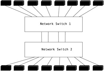 Figure 4.2: A complex cluster network.
4.3 Network SoftwareIn order for applications to use the network, applications need to access the network via a set of software. This software stack will provide a range of functionality, and will exist in a number of forms. At the highest level, there are communication libraries, for example, MPI implementations. These are typically used by applications because they provide a transport and platform independent interface to communication. (These libraries won't be discussed in detail in this chapter; see Chapters 8–11 for details.) At a slightly lower level, protocol stacks are used. These protocol stacks provide transport properties like reliable message delivery, ordered message delivery, message framing, and flow control. The lowest level of network software is the driver layer. Network drivers interact directly with network interfaces to control transmission and receipt of packets on the network.
4.3.1 Network Protocols
Network protocols are a series of procedures used to setup and conduct data transmissions between a group of machines. Such protocols abstract the physical transmission medium to provide some portability to applications. Protocols are used to provide various properties to network communications sessions. Note that not all protocols provide all of these properties, and the following list is by no means exhaustive.
-
Media contention: work around collisions and other physical errors.
-
Addressing: A station addressing scheme that is network layer independent.
-
Fragmentation: A means to break down messages into smaller pieces (called datagrams) for transmission, and reassemble them at the receiver.
-
Reliable delivery: A means for the client to determine if transmission completed properly or an error has occurred.
-
Ordered delivery: Messages are delivered in order to the application from end to end.
-
Flow control: Transmission can be slowed to improve performance or prevent the exhaustion of resources at the destination or along the route to the destination.
Most applications will actually use a combination of network protocols in the course of communications. This means that all protocols do not need to provide all of the above properties. For example, the IP protocol only provides an addressing scheme and message fragmentation: the IP protocol provides an addressing scheme that allows a message to be delivered to another end station and that it is fragmented and reassembled if necessary. Most IP applications also use either TCP or UDP. TCP is used when reliability and ordered delivery are desired. The following are descriptions of a number of common network protocols and the properties they implement.
Ethernet provides media collision detection and avoidance. The Ethernet protocol also provides an addressing scheme. Each client uses a 48-bit address, assigned by the vendor of its network interface.
IP is a protocol that provides the features of addressing and fragmentation. Addressing is implemented in the following way. Each client address has a 32 bit address, broken into a network address and a host address. Network addresses are used to route packages from one network segment to another. Fragmentation is implemented using a identification field in the header. IP also includes a header field that specifies the transport layer protocol as well. This will in most cases be either TCP or UDP, but other protocols can be used as well.
The IP protocol must be adapted to the underlying physical network type. IP addresses must be able to be mapped to physical network addresses. In the case where IP is used on top of Ethernet, the address resolution protocol (ARP) is used to determine the Ethernet address of the intended recipient. This process consists of a broadcasted query for the MAC address of an IP address. The owner of that IP address will respond with the MAC address. This value is cached. At this point, IP can be used on top of Ethernet transparently. See
Section 5.2 for a more detailed discussion of IP, TCP and UDP.
TCP specifies a set of steps required to establish a communication session. Once this is established, it provides reliable, in-order delivery of messages.
UDP provides about the same functionality as IP. It is generally used so that an application can implement its own network protocol for reliable delivery of messages. UDP is also used in cases where reliable message delivery is not as important as low latency or jitter. UDP is frequently used for streaming audio and video.
GM is the driver, firmware, and user-space library used to access Myrinet interfaces. It provides all of the properties necessary to use the network for reliable communications. Addressing is implemented in GM using interface hardware addresses and a routing table that exists on each node. This routing table has a set of source routes for all nodes on the network. Fragmentation is not necessary, as GM messages are not limited in size. GM also implements reliable, in-order message delivery. Because of the switched nature of myrinet switch complexes, media contention is not an issue.
The kernel driver providing support for GM on Myrinet interfaces also provides Ethernet emulation. This means that protocols like Ethernet and IP (TCP and UDP) can be run over Myrinet hardware.
4.3.2 Network Protocol Stacks
Network protocol stacks are the software implementations of the network protocols mentioned in the previous subsection. These implementations are typically operating system specific. Many of these are implemented inside of the kernel, but this is not universally the case. These stacks provide a syscall interface for user-space programs. The most common example of this interface is the socket interface used by all IP-based protocols. An application will set up a socket, and then send and receive data using this socket. All of these function calls are implemented as system calls. The network stack uses network drivers to actually send and receive data. The purpose of the syscall layer is to provide portability between different implementations of facilities provided by the kernel. This layer is tightly coupled with network drivers, as it is the sole consumer of their functions.
4.3.3 Network Drivers
Network drivers are the software that allows network interface hardware to be used by the kernel, network protocol stacks, and ultimately user applications. Network drivers have a few responsibilities. First, the driver will initialize the network card, so that it can be enabled. This setup consists of internal setup like on-card register initialization, but also includes external setup like link auto-negotiation. After these steps are complete, the network hardware should be initialized. This does not mean the interface is completely configured, as some configuration processes like DHCP use the network interface itself to configure settings like IP addresses.
The driver also provides functions necessary to send and receive packets via the network. The send functions are typically called from a protocol stack. The set of transmission steps is as follows: an application makes a system call, providing data to be sent. This data is processed by the network protocol stack. The protocol stack calls functions provided by the driver to copy the data across the I/O bus and actually transmit the data.
When receiving data, the network interface will receive data from the network. It will then do some amount of processing of the data. This processing varies from card to card. Some cards implement parts of the protocol stack in hardware in order to improve performance. When the card is finished processing the packets received from the network, it causes an interrupt. This causes the kernel to call functions defined in the network interface driver. These functions are called interrupt handlers. An interrupt handler will copy the data from the network interface to system main memory, via the I/O bus. At this point, the network protocol stack finishes processing the packets, and copies the data out to the application.
The process of servicing interrupts is very invasive; it typically causes other operations to be preempted. Under high network receive load, this causes the primary computational task of the system to be frequently stopped. As context switches are not free, this constant switch comes at a high performance price. In order to address this issue, most high-end (gigabit and custom network) NIC manufacturers have implemented interrupt mitigation, or coalescing strategies. This means that the NIC will buffer some number of processed packets before issuing an interrupt. This means that instead of interrupting after every packet is processed, the NIC may only issue an interrupt after 10 or 100 packets. This allows the spend less time switching between the network and computational task, and more time executing the user's application. See
Sections 5.5.4 and 5.5.5 for more information about driver performance settings and techniques.
4.3.4 Network Software In Action
In general, cluster use is characterized by the execution of parallel applications. These applications consist of many instances of the same application, running on multiple cluster nodes simultaneously. These instances of the application use the system area network to communicate. These messages are typically used for coordination between instances of the parallel application.
When communication occurs, a complex series of actions is performed. First, the application makes a library call to initiate message transfer. This call usually does a variety of things; it will frame the message and potentially split the message into multiple packets if the message size is too large. At this point, the packet is passed to the network driver stack. The data is transferred across the I/O bus to the NIC.
The network controller transmits the packets to the network controller on the intended recipient. The packet reaches receiving network controller, where it is processed by the hardware and processed by the network driver stack. These packets are reconstituted into the original message by the protocol stack, and this message is passed to the application when if calls a receive function in its messaging library.
4.5 Network ChoiceChoosing the appropriate system area network for a cluster can be complicated process. Two factors weigh heavily in this sort of decision. The first is cost. Realistically, most clusters are built with a fixed budget. This means that a higher-priced, higher-performance network will probably come at the cost of needing to purchase a smaller cluster. In many cases, specialized network interconnects can cost upwards of $1000–2000 per node. At this point, this cost approximates the cost of a high performance compute node. This means that building a high-performance network can reduce the cluster size by a factor of two, when working with a fixed budget. As we saw in
Section 1.3.6, a high-performance network can be a very reasonable use of resources because of the greatly improved performance it can provide.
Another important factor is the performance of the network, and accordingly, the cluster itself. Many applications need particular performance properties to function effectively. Serviceability is a third concern. When the scale of a cluster increases beyond 32 or 64 nodes, many low-cost solutions become quite unwieldy, and result in largely unusable clusters. Fundamentally, all of these factors are pieces of the same puzzle: how to get the best value out of a cluster for its intended uses.
If a cluster is being built for a small number of applications, thorough application benchmarking is in order. The spectrum of communication patterns exhibited by application ranges from occasional communication from one node to another, to consistant communication from all nodes to all other nodes. At one extreme are applications that behave like SetiAtHome, wherein compute nodes will infrequently query a master node for a work unit to process for hours or days. At the other extreme are many scientific applications, where nodes will be in constant communication with one or more other nodes and the speed of the computation is limited by the performance of the slowest performing node. As is obvious from the communication pattern description, basically any interconnect would perform admirably in the first case, while the fastest interconnect possible is desirable in the second case.
The range of network options available to clusters ranges from the integrated Ethernet that is included with nearly any computer sold today, to higher speed interconnects with substantially higher costs. Performance varies greatly between these options. Integrated gigabit Ethernet will typically provide 100 MB/s of bandwidth, with latencies measured in the tens to hundreds of microseconds. Cluster interconnects generally provide five to ten times the bandwidth, providing latencies in below ten microseconds. As with many of the technologies described here, the state of the art is a fast moving target. Precise high-end performance figures would be out of date within months; check online sources for up to data figures.
5.1 Cluster Network DesignsJust as many styles of node and network hardware exist, so do a wide variety of cluster network designs. To understand why such variety exists is to understand how the choice of network design directly affects the operation of the cluster as a whole. In general, the motivation for such variation comes from the striving to achieve a perfect balance of usability, performance, and security. As a result, the cluster designer has realized that network design impacts all of these in important ways.
5.1.1 Impact of Network Design
Although it would be impossible to fully enumerate how a cluster network design impacts the overall look, feel, and operation of a cluster, there are some key aspects that are directly and substantially affected.
One of the first issues affected by the cluster network is security. Questions include how secure the system is from outsider attacks, how we maintain security over time, and how the cluster fits within institutional security requirements. The cluster network design should directly address all of these issues since the primary security defenses are often implemented inside the institution's network itself.
The cluster's usability is defined by how users interact with the system and what types of applications will use the cluster. Application requirements impact every aspect of the cluster design, and the cluster network is no exception. If the cluster is designed to run a single application, the designers can make very focused decisions about how the user(s) can employ the machine. If the cluster is meant to be a general resource for students, researchers, etc., then intuitiveness and ease of use must be considered.
Finally, we cannot overlook the impact of the cluster network design on application performance. The cluster network may impose bottlenecks that could limit the performance of an application. The designer must be aware that some decisions, while bolstering the security and usability of the cluster, can seriously impact the performance of applications.
5.1.2 Example Designs
Over time, cluster network designs have evolved from simple networks of desktops and servers. Modern designs focus more on the specific realm of high performance computing and thus often mirror network designs that large site administrators have been employing for years. The cluster community has built upon this substantial groundwork to generate a wide variety of network topologies. As we examine some common network designs, we should remember that the examples are a small subset of the many possibilities. For each of the following design descriptions, we could imagine a dozen permutations, each having a different positive or negative impact on overall cluster issues.
The first, and probably the simplest, style of cluster is the fully connected system. In this case, all nodes in the system, as well as any front end servers or login machines, are simply connected to the Internet the same way as any non-cluster server or workstation. The major benefit of this design is obvious: very little work is required to initially bring the system online. While the simplicity of such a design is attractive, the users and administrators of these systems must constantly be aware of all the implications. Security, for instance, will be a major concern. Although each node is easily accessed by legitimate users and administrators from anywhere on the Internet, each system is equally accessible to malicious outside attackers.
A simple optimization would be to reduce the number of systems visible to the Internet. Such a system would have a publicly available front end login machine, with all other nodes hidden behind a firewall and only visible from that front end machine. A user would log into the front end and then have access to cluster nodes. Although such a design provides tighter system security, we still have a machine visible to the Internet. Internet visibility is inherently problematic, but certainly does not make the system impossible to tightly secure. One interesting disadvantage of this design is that users whose work requires compute resources to be Internet accessible are unable to use such a system.
Going one step further, measures could be taken to completely block all access to compute nodes, even from the user. The user would log into a cluster front end (login) machine and would perform local operations such as compilation or preliminary testing. When the user's program is ready to be run on the cluster, it is submitted as a job to the cluster scheduler. When sufficient compute nodes become available, the scheduler runs the job on the user's behalf. Notice, in this design, the cluster nodes are never directly accessed by the user. The nodes are therefore completely hidden to all entities except the scheduler and other cluster services. We further could extend this concept by disallowing users access to the front end machine. Instead, the cluster would only accept jobs from a meta scheduler.
One interesting design simulates a large multi-processor computer with a single system image on a Linux cluster. By running custom operating systems, nodes become nearly invisible to users or outside influences. On such a system, users would employ an OS level mechanism present on the login machine (which may or may not be externally visible) to run processes on the cluster compute nodes. The biggest advantage of this design is ease of use for the application user. The user interface to a single system image avoids the common problems of managing remote processes. Disadvantages may arise when a user needs direct access to the compute nodes, which is prohibited by the nature of the system.
Cluster designers have put tremendous efforts into creating network topologies suited to their individual needs. Many designers have made their experiences and technologies available for other cluster designers to use. For some real life examples of cluster designs, see
Chapters 6, 18, and 20.
Armed with an awareness of various cluster network configurations, as well as some of the most importantly impacted issues, the cluster designer can embark on designing a network that optimally addresses individual needs. However, knowing the issues and possibilities at hand is only the first step. We must understand the simplest case of cluster network designs and some of the concepts surrounding their construction. In the sections that follow, we introduce customary communication protocols and give a short overview of Linux networking concepts and services, before delving into the construction of a simple cluster network.
5.2 Internet Protocol StackSimple Beowulf clusters are built with commodity networking hardware, typically Ethernet based, and communicate using standard networking protocols such as TCP/IP. Before examining UNIX networking concepts and services, as well as the configuration of a simple cluster, it is important that you understand the protocols involved in network communication. Understanding the protocols will be necessary when performing advanced configuration, troubleshooting problems or attempting to improve performance.
Networking protocols are built, at least conceptually, in layers.
Figure 5.1 depicts the layers involved in TCP and UDP communication. In the paragraphs that follow, we will describe the layers from the bottom up, focusing on details important to our later discussions. While a full discussion of IP networking is beyond the scope of this chapter, the interested reader will find that [
28,
110] discuss the topic in great detail. In addition, a more general discussion of network hardware, software, and protocols can be found in
Chapter 4.
A combination of the network interface card and the associated driver is responsible for sending frames out to other devices on the local area network. The maximum amount of data that can be placed in a frame is otherwise known as the maximum transmission unit (MTU). The MTU for an Ethernet device depends on which specification the device implements, but most devices have a MTU of 1500 bytes. Some newer Ethernet devices can be configured to send and receive jumbo frames, resulting in a MTU as large as 9000 bytes. Jumbo frames and their implications will be discussed further in
Section 5.5.4.
The Internet Protocol (IP) is the building block for TCP and UDP. IP is a communication protocol for transferring messages known as datagrams between machines, even machines on different networks. An IP datagram consists of a header plus data. The header contains, among other things, the addresses for the source and destination machines and the length of the datagram (in bytes). The destination address is used by special network devices known as routers to forward (or route) the datagram between networks until the datagram reaches its destination.
Section 5.3.1 contains a more detailed discussion of IP addresses and routing.
The length field of the datagram header is only 16 bits wide. As a result, the combination of the datagram header and data can be at most 65,535 bytes in length. However, as you might have guessed, IP datagrams are transmitted on the underlying network using frames, a network whose MTU is generally much smaller 65,535 bytes. To solve this problem, IP datagrams larger than the MTU are fragmented into a series of IP packets and reassembled by the receiver. In addition, fragmentation may occur if a packet is routed through any network having a smaller MTU.
IP is what is known as an unreliable, unordered, and connectionless protocol. Unreliable suggests that datagrams sent using IP may not arrive at their destination. Although the protocol makes every effort to deliver the datagram, network misconfiguration, resource exhaustion, or outright failure may result in data loss. Unordered indicates that datagrams that do arrive at their destination may arrive in a different order from the one in which they were sent. And finally, connectionless implies that no state is maintained at the sender or the receiver between datagrams.
The User Datagram Protocol (UDP) is a thin layer on top of IP. Like IP, UDP is unreliable, unordered and connectionless. The primary contribution of UDP is the addition of ports. IP only identifies the source and destinations machines, not which application or service was involved in the communication. The port is an integer identifier that allows multiple flows of communication to exist between a pair of machines and ensures that the datagrams are delivered to the appropriate application or service.
The Transmission Control Protocol (TCP), also layered on top of IP, is substantially more complex that UDP. TCP provides a bidirectional connection over which a stream of bytes is reliably communicated. Like UDP, TCP uses ports. A connection is uniquely identified by a four-tuple (source address, source port, destination address, destination port). Using this four-tuple, the TCP layer can locate the structures maintaining the state of the connection.
With TCP, data in the stream is divided into segments for transmission. These segments, plus a TCP header, are encapsulated into an IP datagram. To avoid fragmentation, which can adversely affect performance, the maximum segment size (MSS) is advertised when the connection is formed so that the segment data plus the TCP and IP headers do not exceed the MTU of the underlying network. On a local-area network (LAN), the MSS can be computed by subtracting the size of the TCP header from the network device's MTU.
TCP connections that reach outside of the LAN are more difficult as the MTU of all the networks involved is unknown when the connection is formed. In this case, most TCP/IP implementations assume an initial MTU of 576 bytes, unless an alternative value is specified by the system administrator. A discovery process is then employed to determine a MTU that is acceptable for all networks involved in the connection. Since the primary focus of this chapter is the cluster network, a discussion of wide-area network MTU discovery is unwarranted. However, the interested reader will find introductions to the topic in [
28, 110] and a detailed discussion in
74.
TCP uses a coupling of positive acknowledgments and a sliding window protocol. Positive acknowledgments and data buffering along with timeouts and retransmission provide the reliability. The sliding window protocol allows the sender to have multiple unacknowledged segments outstanding, substantially increase throughput. Additionally, the protocol provides the receiver with the ability to advertise the amount of buffer space available at its end of the connection. By knowing the amount of available space at the receiver, the sender can avoid transmitting more data than can be accommodated by the receiver. This is known as flow control. More detailed discussions of these topics, and TCP as a whole, can be found in [
28, 110, 87].
This concludes our high-level overview of the Internet Protocol stack. Building and operating a Beowulf cluster by no means necessitates mastering these protocols; however, a basic understanding is required. After all, it is these protocols that enable network communication. In the coming section, we will discuss a series of networking concepts and services which are built upon these very protocols.
5.3 Networking Concepts and Services
Before constructing a cluster, it is important to understand the concepts and services that are involved in UNIX networking. This section presents the basics in preparation for the step-by-step configuration of a simple cluster coming up in
Section 5.4. Additional information on the topics presented here can be found in
[56].
5.3.1 IP addresses
Each node in the cluster must be assigned a unique IP address. IP addresses consist of 32 bits or four octets[
1] and are usually expressed by writing each octet in decimal and separating the octets with a decimal point. This is known as dotted decimal notation. As an example, 192.168.13.24 is a valid IP address.
A netmask is used to split the IP address into two parts: the network address and the host address. The netmask expresses how many of the high-end bits of an IP address are part of the network address. The low-end bits of the IP address then form the host address. Using the previous example address of 192.168.13.24, asserting a netmask of 255.255.255.0 would mean that the network address is 192.168.13.0 and the host address on that network is 24. Two special host addresses are reserved and may not be used to identify an actual host. All bits turned off (or zero) is the address of the network, and all bits turned on (or 255 in our example) is the network broadcast address.
Hosts that share the same network address are generally part of the same physical network and can talk directly to each other. Hosts on different networks require a router to talk to each other. The router uses the network portion of the destination IP address to determine onto which physical network link to forward the data packet. In complex networks, the data packet may be forwarded by several routers before it finally reaches the destination network and ultimately the destination host. To begin this forwarding process, the sending host must know the address of the router on its local network. The address of this router is know as the gateway address.
Not all IP addresses are routable to the Internet. Three address ranges have been reserved for private (internal) networks:
-
10.0.0.0 - 10.255.255.255
-
172.16.0.0 - 172.31.255.255
-
192.168.0.0 - 192.168.255.255
These address ranges may be used by clusters that either have no need to communicate with Internet resources or are hidden behind a firewall that does network address translation (NAT). Discussion of network address translation is beyond the scope of this chapter; however, the interested reader will find the topic covered in
[127].
5.3.2 Hostnames
In addition to an IP address, each node in the cluster will require a unique name. Names generally come in two forms: short and long. The long name is used when referring to the host from outside of the local domain (or subdomain) in which it is present. The long name for the first node in our Beowulf cluster might be bc1-001.phy.myu.edu. Notice that the long name is hierarchical. It refers to the node bc1-001 in the phy (short for the Physics department) subdomain which is part of the myu.edu domain. The short name, bc1-001, is often used when referring to the node from within the local subdomain, the Physics department.
With clusters, it is common practice to name the cluster nodes after their host addresses. For example, nodes in a 128 node cluster with IP addresses ranging from 192.168.13.1 through 192.168.13.128 and a netmask of 255.255.255.0 might be named bc1-001 through bc1-128. Computer scientists who prefer to begin counting their nodes from zero should recall that host address zero is reserved for the network address (192.168.13.0 in our example). To avoid having the host address and the node name differ by one, it is best to number nodes starting from one
[108].
An additional side effect to starting the node number and host address of the first node at one is that the gateway address must follow that of the nodes. To allow room for expansion, the gateway address is generally given the maximum available host address. Remember, that the maximum host address is reserved for the network broadcast address, so the gateway address is generally assigned the address just prior to the network broadcast address. In our continuing example, the gateway address would be 192.168.13.254.
5.3.3 Name resolution
Given a set of hostnames and IP addresses for the nodes in the cluster, a mechanism is needed to map from one to the other. For a small number of nodes, this can be accomplished with a hosts file ('/etc/hosts'). The hosts file will include a line for each node in the cluster. Each line contains the IP address of the node followed by the names the nodes is known by, usually the long name first followed by the short.
The hosts file traditionally contains one additional mapping from the names localhost and localhost.phy.myu.edu to 127.0.0.1. The address 127.0.0.1 is tied to the loopback device driver that funnels all messages sent from it back to the same host. The combination of the loopback device and the mapping in the hosts file allows a host to communicate with itself as though it were any other host on the network simply by using the name localhost.
One caveat of using a hosts file is that it must be replicated and kept current on every node in the cluster. However, for most environments, the hosts file does not change that often. A master copy can be kept on one node of our cluster and then pushed to the other nodes when changes are made. This push operation would be tedious to do by hand, but it is not very difficult to write a script to copy the hosts file to the other nodes using a program like scp. A brief description of scp can be found in
Section 5.3.5.
Chapter 6 describes tools that can handle all of these setup steps for you; the material in this section describes some of the operations that those tools must perform and provides some background for understanding how those tools work.
As an alternative, the Network Information Service (NIS) exists to perform this type of replication automatically. NIS allows the system administrator to manage a single copy of important files like the hosts file on one node designated as the NIS server. The other nodes, acting as NIS clients, obtain the host information from the NIS server as necessary.
In addition to maintaining a single copy of the hosts file, NIS can also be used to propagate account ('/etc/passwd') and group ('/etc/group') information, as well as other important system files. A more detailed explanation on the capabilities of NIS can be found in
[109]. An example configuration of a NIS server and clients will be shown in
Section 5.4.
Another option for avoiding the replication of the hosts file is the Domain Name Service (DNS). DNS differs from NIS in two major ways. First, its sole purpose is to return information about a host or domain. Second, it performs resolution for hosts outside of the local domain. DNS is by design a scalable distributed database capable of handling name resolution for the entire Internet. Further information on DNS and Berkeley's implementation (BIND) can be found in
[1].
DNS and NIS are designed to work together. It is not uncommon to use NIS for resolution of local hostnames and DNS for resolving names external to the local domain (or subdomain).
5.3.4 File sharing
In most networked computing environments, the ability to share files with other machines on the network is extremely useful. Such a capability allows system administrators to install a software package once an make it accessible to a set of machines. File sharing also allows users to create a file on one machine and access it from a variety of other machines on the local-area network. For Linux environments, this file sharing capability is traditionally provided by the Network File System (NFS).
File sharing is useful on Beowulf clusters for the same reasons. Application programs built by users typically reference libraries from other software packages. If these software packages use shared libraries, ones that are dynamically loaded at runtime, then those libraries must be accessible on all nodes where the application is being run. Thus the system administrator has two choices: installing the necessary packages on each of the nodes or using a network based file system like NFS to make the packages available to each of the nodes.
Likewise, the typical user of a Beowulf cluster will wish to run their application on several nodes, perhaps simultaneously. Most users find copying their application's executable and input data files to each node before executing the application undesirable. Instead, they would like to build their application on a single machine, construct any necessary input files on that same machine, and have the executable and input files automatically available on all nodes of the cluster. Again, a file sharing system like NFS can help. Using NFS, the users' home directories can be exported from one machine to each of the cluster nodes, allowing access to these home directories from anywhere in the cluster. A detailed explanation of NFS and its capabilities can be found in
[109].
5.3.5 Remote access
The purpose of building a Beowulf cluster is to run user applications. In a networked computing environment, users typically do not have access to the console of all the compute resources. Even if they did, it is much more convenient to access those resources from the workstations present on their desktops. Clusters are simply an array of compute resources with which users wish to interact, execute programs, and share files.
A traditional UNIX system has programs like telnet and rlogin to establish an interactive terminal session with remote compute resource over the network. In addition, rsh executes commands on the remote resource without user interaction, and rcp transfers files between a local and remote resource when direct file sharing is not available. The last two commands are especially powerful because they allow complex remote operations to be scripted and executed without user interaction.
The problem with all of these commands is security. None of the data transferred between the local and remote hosts is encrypted, thus allowing the data to be easily read if captured by someone monitoring network traffic. While a user might not care if someone saw their interactions with a remote resource, telnet transmits the user's password over that same unencrypted channel. All users should care if their passwords are visible to potential outside attackers.
The rsh and rcp commands do not send passwords, making them somewhat more secure. Instead they use host based authentication. If the host is listed in the system's or user's authorized hosts file on the remote machine, then the command is allow to proceed. The rlogin command will also use host based authentication if possible; but, if the host is not authorized, rlogin will ask for the user's password.
Clearly, host based authentication is preferable to sending a password in clear text. However, host based authentication is not without its problems. First, all hosts on the local network must be strictly controlled. Physical security is important. If a malicious host is allowed to attach to the local network, it can be configured to appear as an authorized host, thus compromising security. Second, access to the authorized hosts files must be tightly controlled. If these files can be compromised, so too can the machines for which they control access. Hence, many system administrators disallow the use of user controlled authorization files (i.e., '~/.rhosts').
SSH, or the Secure Shell, was designed as a replacement for the previously mentioned remote access tools. However, SSH is more than a just remote execution shell. It is a suite of tools utilizing public-private key based authentication and modern day encryption to provide a secure means of remote access. As might be expected, it contains programs like slogin, ssh, and scp to replace their less secure counterparts. SSH also contains tools for creating and managing authentication keys, the foundation of its security. In addition, recent implementations like OpenSSH also provide a secure form of FTP.
SSH uses host authentication keys to verify that a host is the expected host and not a malicious decoy. During connection establishment, these keys are used to verify that the connection is with the expected remote host before vital information, such as the user's password, is sent. If host based authentication is employed, the connecting host can be verified before authorization is granted. It is still important to strictly control which hosts are authorized and to disallow user controlled authorization files; but, on a properly configured system, SSH's use of host authentication keys substantially reduces the security risk associated with host based authentication.
SSH can also use authentication keys as a replacement for user passwords. The advantages may not be immediately apparent; however, when combined with the SSH agent, user authentication keys can be very powerful. A more detailed discussion of authentication keys, both host and user, and the SSH agent will be presented in
Section 5.4.6.
5.4 Simple Cluster Configuration WalkthroughNow that we have discussed basic UNIX networking concepts and services, and briefly described the protocols involved in network communication, it is time to walk through the configuration of a simple cluster. Since we cannot cover the variety of Linux distributions in existence, we have chosen to use Red Hat Linux 9 for our example. If you are using a different Linux distribution, the concepts should be same, but the exact commands and files may be different. Note that
Chapter 6 describes tools that automate many of the following steps; we are describing them here to provide an understanding of the steps involved in setting up a cluster network.
Our example cluster consists of eight nodes. As in our previous examples, to avoid using IP addresses that may belong to an existing domain, we place the nodes of our cluster on a private network with a network address of 192.168.13.0 and a netmask of 255.255.255.0. The gateway address to our router is 192.168.13.254, the domain is phy.myu.edu, and our nodes are named bc1-01 through bc1-08. The cluster configuration is depicted in
Figure 5.2.
When installing Red Hat Linux 9 on each of the eight nodes, we used the standard "Workstation" install with one exception. We included the NIS server package ypserv on the first node. Later, we will run a NIS server on bc1-01 for the purposes of propagating system information like accounts and hostname to IP address mappings. Although the NIS hosts map is used for resolving names local to our cluster, we assume that a DNS server exists at 192.168.1.1 to obtain information about hosts outside of our cluster network. In addition to NIS, we will also run a NFS server on bc1-01 to provide each user access to a common home directory accessible from all of the nodes.
5.4.1 Hostname and gateway address
We begin by setting the hostname and gateway address on each of the machines. These parameters may have been set during the installation of the operating system; in which case, we need only verify that they are correct. Both of these parameters are set in '/etc/sysconfig/network'. The contents of this file for the first node of our cluster should be as follows.
Alterations made to this file do not take effect immediately; however, the changes should be realized the next time the system is rebooted. If you had to make changes, it is recommended that you reboot now. This can be accomplished by executing shutdown -r now.
Notice that the long name is used in the HOSTNAME setting. Use of the short name for this setting is discouraged as doing so makes it difficult, if not impossible, for applications and libraries to properly identify the local machine in the global namespace. This can cause some programs to behave incorrectly or fail altogether.
5.4.2 Network interface configuration
Next, we need to configure the IP settings for the network interface on each of the nodes. The network interface settings can be changed using two different methods. The first is to use a program like netconf; the second is to edit the configuration file directly. We will edit the configuration file, '/etc/sysconf/network-scripts/ifcfg-eth0', so the exact location of the settings is clear. The contents of the configuration file for the first node of our cluster should be as follows.
The settings on the other nodes are largely the same. Only the IPADDR setting needs to be adjusted.
Alterations to the network interface configuration file should only be made when the interface is disabled, accomplished by running ifdown eth0. Once the changes are complete, ifup eth0 can be run to re-enable the interface with the new settings.
5.4.3 Name resolution
For our cluster, the hostname to IP address mappings are as follows.
To avoid a substantial amount of repetitive typing, the complete set of mappings need only be entered into the '/etc/hosts' file on bc1-01. Later, in
Section 5.4.7, we will configure NIS to provide this information to the other seven nodes. The '/etc/hosts' file on the remaining nodes should consist only of the following entry.
In addition to the hosts file, we need to configure the service that resolves names (the resolver for short) on each node of the cluster. The configuration file, '/etc/resolv.conf', must contain the following.
The resolver configuration file contains two important pieces of information. The first is the IP address of the DNS server used to resolve names not found in the hosts file or the NIS hosts map; the second is the search list for hostname lookup. If a short or incomplete hostname is supplied, entries in the search list are individually appended to the hostname. For example, if the system were attempting to resolve the hostname foo, it would append phy.myu.edu and then perform a DNS query for foo.phy.myu.edu.
5.4.4 Accounts
At this time, we need to create accounts for the users of our cluster. It is recommended that each user have his own account, including the system administrator(s). While the administrator already has access to the root account, that account should only be used to perform administrative tasks. Use of the root account for non-administrative tasks is frowned upon because that account is unchecked, allowing for unintentional damage to the operating system. For more details on account management, see
Section 13.6.
Users may be added to the system with the adduser program. Running adduser <username> creates an entry for the user in the account information and shadow password files, '/etc/passwd' and '/etc/shadow' respectively. The adduser program also adds a group for the user in '/etc/group' and creates a home directory for that user in '/home/<username>'. Usage information about the adduser program can be obtained by running man adduser.
The creation of user accounts and home directories across all of the nodes in the cluster could be handled by running adduser on each node for each user. However, this repetition is tedious and requires care so that the user and group identifiers are consistent across all nodes. Alternatively, we could create a script which uses scp to replicate the appropriate system files and ssh create the necessary home directories on each node. Instead, since we are already using NIS to provide the host map, we will configure NIS to also provide account and group information to the other seven nodes. Additionally, we will use NFS to make the '/home' directory on bc1-01 accessible to the remaining nodes. NIS will be configured in
Section 5.4.7 and NFS in
Section 5.4.8.
By default, adduser creates the account with a bogus password entry; thus effectively disabling the account. To enable the account, run passwd <username> to set an initial password for the account. Usage information about the passwd program can be obtained by running man passwd.
Unlike normal user accounts, NIS does not publish account information for the root user, and NFS is not configured to export the root user's home directory, '/root'. Doing either is considered a security risk as it may allow a malicious user to obtain privileged information and compromise one or more nodes of the cluster. Instead the root user has a separate entry in '/etc/passwd' and '/etc/shadow' and a separate home directory on each cluster node. While these restrictions affect the ease with which the root user can change its password or share files between machines, the security of the cluster as a whole is improved.
5.4.5 Packet filtering
As a security measure, the Linux kernel has the ability to filter IP packets. Among other things, packet filtering allows the system administrator to control access to services running on a machine. By default, Red Hat Linux 9 uses packet filtering to block remote access to most services including SSH, NFS and NIS. This default configuration presents a problem for a cluster environment where remote execution, file sharing and collective system administration are critical.
To allow SSH, NIS and NFS to function, we must add a few new packet filtering rules to each node of our cluster, allowing SSH, NFS and NIS to function. For Red Hat Linux 9, packet filtering rules are specified in the file '/etc/sysconfig/iptables'. Into this file, we insert the following rules before the first line that starts with -A INPUT.
Once those changes have been made, the following command must be executed so the changes will take effect.
The first rule we added tells the packet filter to allow new TCP connection requests made to port 22, the port monitored by sshd. With this rule in place, ssh and scp can be used to access the nodes in our cluster from any other machine on the network, including those not part of the cluster. If we were using routable addresses and our network was Internet accessible, any machine on the Internet could attempt to access our cluster nodes. This accessibility might appear to be a security concern; but, the connecting entity must know the name of an existing account and the associated password to obtain access, both of which SSH encrypts before transmitting them over the network.
The second and third rules tell the packet filter to accept any packets from any machines on the cluster network. These rules allow NFS and NIS to function between nodes in the cluster. The rules may seem unnecessarily liberal because they allow all UDP and TCP packets to pass. However, the NIS services and the network status monitoring service used by NFS are dynamically assigned ports by the portmap service. Because these port values are not known in advance, they cannot be explicitly specified in our packet filtering rules. In addition, we don't want to prevent applications running across nodes of the cluster from being able to communicate with each other. Therefore, we allow packets to freely flow between machines on the cluster network while still blocking potentially security threatening traffic from the outside.
More information about Linux firewalls and iptables can be found in
Section 5.6.2.
5.4.6 Secure shell
The OpenSSH package is installed automatically with Red Hat Linux 9, which means the SSH remote access clients like ssh and scp are available to users immediately. The SSH service sshd is also available and started by default. Once the packet filtering rules discussed in
Section 5.4.5 have been applied, the root user should be able to remotely access any of the nodes in the cluster. This ability can be tremendously useful when one needs to replicate configuration files across several nodes of the cluster or to restart a service without being at the console of the specific node.
Initially, non-root users will only be able to remotely access bc1-01. This restriction is lifted once NIS and NFS have been configured and enabled, thus providing account information and home directories to other nodes in the cluster. The configuration of NIS and NFS are discussed in
Section 5.4.7 and Section 5.4.8 respectively.
The first time the sshd service is started, authentication keys for the host are generated. The keys for the remote host are used during the establishment of a SSH session, allowing the client (e.g., ssh) to validate the identity of the remote host. However, the validation can occur only if the client knows the public key of the remote host to which it is trying to connect. When the public key of the remote host is unknown, the user is notified that the authenticity of the remote host could not be verified. The connection process then continues only if the user explicitly authorizes it. If the user agrees to continue establishing the connection, the client stores the name of the remote host and its public key in '~/.ssh/known_hosts' on the local machine. The stored public key is used during the establishment of future connections to validate the authenticity of the remote host.
To prevent the user from being questioned about host authenticity, the system administrator can establish a system-wide list of hosts and their associated public keys. This list is placed in the '/etc/ssh/ssh_known_hosts' file on each of the nodes and any other machines that are likely to remotely access the nodes. This approach has one other advantage. If a node is rebuilt and new authentication keys are generated, then the system administrator can update the 'ssh_known_hosts' files. Such updates can prevent the user from receiving errors about host identification changes and potential man-in-the-middle attacks.
The contents of the 'ssh_known_hosts' file can be generated automatically using ssh-keyscan. To use ssh-keyscan, we must first create a file containing a list of our cluster nodes. Each line of this file, which we will call 'hosts', should contain the primary IP address of a node followed by all of the names and addresses associated with that node.
Once the 'hosts' file has been created, the following command will obtain the public keys from each of the nodes and generate the 'ssh_known_hosts' file.
The 'ssh_known_hosts' file needs to exist on each node of the cluster. While the above command could be executed on each of the nodes, regenerating the contents each time, it is also possible to use scp to copy the file to each of the remaining nodes.
At this point, the client tools are able to validate the identity of the remote host. However, the remote host must still authenticate the user before allowing the client access to the remote system. By default, users are prompted for their passwords as a means of authentication. To prevent this from happening when access is from one cluster node to another, host based authentication can be utilized. Host based authentication, as discussed in
Section 5.3.5, allows a trusted client host to vouch for the user. The remote host uses the public key of the client host, found in the file we just generated, to verify the identity of the client host. Enabling host based authentication requires a few configuration changes on each of the nodes.
The sshd serv ice must be configured to allow host based authentication by changing, the following parameters in '/etc/ssh/sshd_config'.
The first parameter enables host based authentication. The second parameter disables the use of the user maintained known host file, '~/.ssh/known_hosts', when host based authentication is performed. This change allows the system administrator to maintain strict control over which hosts can be authenticated and thus authorized. The third parameter allows the user maintained authorization file, '~/.shosts', to be used when determining whether or not a remote host is authorized to access the system using host based authentication. This is largely provided for the root user for whom the system maintained file, '/etc/ssh/shosts.equiv', is not used. While utilizing user authorization files could be considered a security risk, the change to the IgnoreUserKnownHosts parameter prevents the user from authorizing access to any hosts not listed in the system controlled '/etc/ssh/ssh_known_hosts' file. But, if host based authentication is not desired for the root user, then the third parameter should be left at its default value of "yes".
Once the sshd configuration file has been updated to enable host based authentication, the system authorization file, '/etc/ssh/shosts.equiv', must be created. That file simply consists of the hostnames of machines trusted by the local host. For our cluster, the file should contain the following.
If host based authentication is to be used to allow a client to vouch for the root user, this same list of hostnames must also be placed in the root user's authorization file, '/root/.shosts'. Again, scp can be employed to push copies of these files to each of the nodes.
Now that the sshd service has been configured and the list of authorized hosts properly established, the sshd service must be restarted. This is accomplished using the following command.
In addition to changing the service configuration file, a small change must be made to the client configuration file, '/etc/ssh/ssh_config'. The following line should be added just after the line containing "Host *".
This option tells the client tools that they should attempt to use host based authentication when connecting to a remote host. By default, they do not.
Users, including the root user, also have the ability to create authentication keys which can be use in place of passwords. Such keys are generated with the command ssh-keygen -t rsa. By default, the public and private keys are placed in '~/.ssh/id_rsa.pub' and '~/.ssh/id_rsa' respectively. The contents of the public key can be added to '~/. ssh/authorized_keys' on any machine, allowing remote access to that machine using the authentication keys.
The ssh-keygen command will allow keys to be generated without a passphrase to protect the private key. Users often generate unprotected keys simply to avoid having to reenter the passphrase with each remote operation. However, this practice is not recommended as it substantially weakens the security of any machine allowing public key authentication. Instead of using unprotected keys, a SSH agent can be established to manage the private key(s) of the user for the duration of a session. The passphrase need only be typed once when the private key is registered with the agent. Thereafter, remote operations can proceed without the continual reentry of the passphrase; but, the private key is still protected should a malicious user obtain access to the file containing it.
From the shell, the agent is often used in the following manner.
The first command starts the agent and then begins a new shell. The second command adds the root user's private key to the set of keys managed by the agent. In this case, only one key is managed by the agent, but more could be added through subsequent invocations of ssh-add. After the agent has been started and the private key has been registered, the root user may execute various client commands attempting to access to one or more remote machines. If the user's '~/.ssh/authorized_keys' file on the remote host contains root's public key, the client command will proceed without requesting a password or passphrase. The final command, exit, causes the shell and thus the agent to terminate.
A general discussion of SSH usage, configuration and protocols can be found in
[11], although the details involving OpenSSH are somewhat out of date. Information specific to OpenSSH commands and configuration can be found in the manual pages installed with Red Hat Linux 9 and on the OpenSSH website,
www.openssh.org. Links to IETF draft documents describing the SSH protocols can also be found on the OpenSSH website.
5.4.7 Network Information Service
Now that the IP packet filter has been configured in a way that allows our services to function, and we have introduced the finer points of SSH, we will proceed with configuring NIS. On each of the nodes, the following line must be added to '/etc/sysconfig/network'.
This line tells the NIS services the name of the NIS domain to which our nodes belong. The NIS domain name can be different than the Internet domain in which the nodes reside (phy.myu.edu). The NIS domain name should identify the group of machines the domain is servicing. In our case, this NIS domain is used only by our first Beowulf cluster. Therefore, we use the domain name bc1.phy.myu.edu to avoid conflicts with other NIS domains that might exist on our local network.
Once the NIS domain has been set on each of the nodes, we must prepare bc1-01 to run the NIS server. Before enabling the server to export information, we must secure the server so that only hosts in our cluster can obtain information from it. Entries in the '/var/yp/securenets' file accomplish this. For our cluster, this file (on bc1-01) should contain the following entries.
Now we are ready to configure and run the NIS server. To begin, we edit the '/var/yp/Makefile' file on bc1-01. We need to comment out the existing line that begins with "all:" and add the following line before it.
This line lists the information sources that we desire NIS to export to the client nodes. NIS maintains a set of databases, known as maps, separate from the source files. To build the maps, the following commands must be executed on bc1-01.
Since '/etc/networks' does not exist on Red Hat Linux 9 installations, the first command creates the file, adding the loopback network as an entry. The next three commands start the services needed by a NIS server. And the last two commands build the actual maps.
The previous commands started the necessary NIS services; however, they did not configure the system so the services would be automatically started at boot time. To accomplish this, we must adjust the runlevel associated with the services. The following commands tell the system to automatically start the services when booting the system. Remember, these commands should only be executed on bc1-01, the system running the NIS server.
Now that we have a running NIS server, it is time to configure the clients. The NIS client service ypbind will be run on all of the nodes in our cluster, including bc1-01. The following commands start the client service and configure the operating system so the service is started automatically when the system is booted.
To make the operating system use NIS when looking up information, we must update the name service switch configuration file, '/etc/nsswitch.conf', on each of the nodes. The entries that follow should be modified accordingly.
When the source files on the server are modified, the NIS maps are not automatically updated . Therefore anytime a new account or group is added or the hosts file is updated, the maps need to be rebuilt. To rebuild the maps, the following commands must be run on bc1-01.
Once the maps are rebuilt, any updates are available to all nodes in the cluster.
The exception to the maps not being immediately updated is the changing of a user's password. If the password is changed using the yppasswd program, the yppasswdd service immediately updates both the NIS maps and account files on bc1-01, making the updated password immediately available to all nodes in the cluster. yppasswd may be run from any node that is part of the NIS domain.
A small problem exists with regards to the NIS client and the sshd service. If sshd is started before ypbind, as it was in our example, then sshd will not use NIS services to obtain account information. Therefore users will not be able to remotely access bc1-02 through bc1-08 until sshd is restarted. The service may be restarted by executing
on each of those nodes. A similar problem will occur if bc1-02 through bc1-08 are rebooted and bc1-01 is not online or is not running the NIS server. The ypbind service will fail causing sshd not to use NIS even if ypbind is started later. So, as a general rule, if ypbind is manually started, sshd should also be restarted.
5.4.8 Network File System
Now that the NIS server and clients are running, the next task is to configure the NFS server and clients, thus allowing users access to their home directories from any of the cluster nodes.
We will begin with configuring the server on bc1-01. To export the user home directories, the following line must be added to the file '/etc/exports'.
This line tells the NFS server that any machine on our cluster network may access the home file system. Once the file has been modified, the NFS service must be enabled and started using the following commands.
Next we need to configure the other seven nodes to mount the '/home' directory on bc1-01. Mounting is the UNIX term for attaching a file system space, whether it be local or remote, into the local directory structure. To express that we wish to have '/home' on bc1-01 be mounted as '/home' in the directory structure present on our remaining cluster nodes, we must add the following line to '/etc/fstab' on all nodes except bcl-01.
Then we execute the following command on each of those nodes to cause the remote file system to be mounted.
You might have noticed that we use the IP address for bc1-01 instead of its host-name when we added the entry to '/etc/fstab'. The reason is that netfs is started before before ypbind when the operating system is booting. If we were to use bc1-01 in place of the address, hostname resolution would fail causing the mount to fail.
The options for mounting a file system exported by NFS are numerous. The manual pages, obtained by executing man fstab and man nfs, provide an explanation of the '/etc/fstab' structure and the available options when mounting file systems via NFS. Additional information can also be found in
[109].
5.4.9 Scripting it
For small clusters, installing the operating system on each node, and performing the previously mention configuration adjustments might not seem so bad. However, for a larger cluster, the task can be annoyingly repetitive and prone to error. Fortunately, several solutions exist.
The Kickstart system, part of the Red Hat Linux 9 distribution, is one such solution. When Red Hat Linux 9 is installed, a Kickstart configuration file is automatically generated during the installation process and stored as '/root/anaconda-ks.cfg'. Starting with the file on created for bc1-01, we can create a 'ks.cfg' file for the other nodes of the cluster. Below is an example configuration file for bc1-02.
| Note |
the lines containing the
network option were broken into three separate lines for printing purposes. The Kickstart system requires that these three lines exist as a single line in the actual 'ks.cfg' file.
|
A few changes have been made to the original 'anaconda-ks.cfg' file in creating a 'ks.cfg' for bc1-02. First, the hostname and IP address, part of the
network option, have been updated. Second, the disk partitioning options clearpart and part have been uncommented informing Kickstart to clear and rewrite the disk partition table with an appropriate set of partitions for bc1-02. Finally, the ypserv package was removed from packages list as bc1-01 is the only node that needs to run the NIS server.
Now that we have created a 'ks.cfg' file, we need to place that file on a floppy diskette. Insert a floppy diskette, preferably a blank one, into the floppy drive and execute the following commands.
The mformat command will destroy any existing files on the diskette, so do not insert a diskette containing files you wish to keep.
Once the 'ks.cfg' file is on the diskette, you should boot the new node with CD-ROM #1 from the Red Hat Linux 9 distribution. When the Linux boot prompt appears, insert the Kickstart floppy and type the following.
If the Red Hat Linux 9 installation system has difficulty detecting the graphics chipset or monitor type for your machine, the following may have to be typed instead.
Since we are installing from CD-ROM, the Red Hat installer will prompt you to change CD-ROMs as necessary. When the process completes, the operating system has been installed on the new cluster node. However, the adjustments we made throughout this section must still be made. But, the process of answering several pre-installation questions, partitioning the disk, and selecting packages has now been eliminated.
Kickstart has a variety of options, many of which we did not use in our example 'ks.cfg'. These options can be used to directly adjust some of the settings described earlier in this section. In addition, Kickstart has the ability to run a post installation script. People with knowledge of one or more UNIX scripting environments should be able to create a post install script to automatically perform the configuration adjustments we made throughout this section. The full set of Kickstart options are described in the Kickstart Installations chapter of
[93].
In
[85], the authors describe a set of tools for rapidly building (or rebuilding) a cluster. These tools consist of a set of Kickstart configuration files and postprocessing scripts. Although their post-processing scripts are run separate from Kickstart, their toolkit is an excellent example of a simple yet effective means of automating operating system installation and network configuration in a cluster environment. More sophisticated approaches are described in
Chapter 6, including NPACI Rocks, which takes advantage of Kickstart to setup a cluster.
5.5 Improving PerformanceThe overall performance of a cluster is very difficult to measure because so many disparate resources must be properly tuned for everything to run at peak performance. Also, different applications may require different tuning parameters to achieve optimal behavior. The cluster network is probably the subsystem that most influences the performance of parallel scientific applications.
Many network performance benefits can be gained at the individual node level, but more still can be uncovered at the network and network design level. When deciding on a specific network technology, the designer must think about performance of the system as well as cost and vendor/OS support. In this section we will discuss some high level network design concepts which increase overall performance of the cluster. In addition, we delve into some low level details involving the tuning of specific protocol and network parameters, thereby giving the reader a feeling for the parts of their network that can be modified to potentially improve application performance.
5.5.1 Offloading Services
One simple method for removing service bottlenecks in a cluster is to offload the service to a dedicated system. In our simple cluster case, we had no machines dedicated to specific tasks. For small systems primarily used for compute bound applications, this may work nicely. But as we increase the number of nodes, the number of users and the complexity of the applications, running services on the compute nodes quickly becomes problematic. Imagine a case where one user's application, running on the node providing NFS service, is fully utilizing the compute and I/O capabilities of that machine. Along comes another user, attempting to run a parallel application with moderate NFS requirements. The result is resource contention for the CPU, disk and network on the NFS server, causing both applications to slow down. If there is one node in a system that has multiple tasks to perform while others have only one task, the potential exists for wasted cycles. The obvious, and often implemented, solution is to offload services to a dedicated service machine so that all compute nodes are identical in the resources they provide to applications. This simple optimization leaves us with a pool of compute nodes distinct from the machine devoted to servicing tasks such as user login, compilation, NFS service, DNS service, etc. If bottlenecks still appear, services may be further split across multiple machines, leaving us with several service nodes, each with their own set of balanced tasks. Service offloading is a very important step towards achieving the goal of maximizing the performance of our cluster. However, the cluster can still have bottlenecks within a specific service.
While not specific to cluster environment, the idea of service load balancing remains a very important concept for cluster network designers. Although the idea of load balancing transfers nicely from more traditional UNIX networks, the specific load characteristics of the same services in a cluster environment can be drastically different. For instance, a traditional UNIX network may happily operate with a single NFS server and a large number of clients; whereas, a cluster with the same number of clients could easily overrun the single NFS server because the intensity and frequency of client accesses is radically different. With this disparity in mind, the cluster network designer should be careful to reevaluate their load balancing experiences with traditional UNIX networks before applying that knowledge to balancing their cluster services.
The specifics of service offloading vary depending on the particular service, but the idea remains the same: identify service bottlenecks (where a single service is being overwhelmed by multiple simultaneous requests) and find a way to offload that specific service to multiple servers so no one server is being overwhelmed. For example, if a NFS home file system server is being overwhelmed, a simple but effective way to lighten the burden is to bring up a second NFS server. The home file system can then be split into two volumes with half the homes served by one machine and the other half served by the second machine. While this technique can work for some services, it can not be used for services that require a synchronized, centralized repository of data. These types of services often have their own mechanisms for dealing with load balancing and should be researched thoroughly before attempting to make any adjustments.
Another case where the "splitting data in two" technique fails is when a single job places high demands on a single service, overloading the associated server. For instance, if a user's job places heavy demands on a single NFS server from many nodes, that job can overload the server. Since there is only one canonical data source, we cannot employ our "split into two" method without introducing serious synchronization problems. As it turns out, this case highlights an inherent scalability problem with the NFS service, which is not easily overcome. In such a situation, we may have to employ more powerful, better scaling solutions to the problem. To rectify this situation, we would likely move to a parallel file system, such as PVFS (see
Chapter 19), which scales by splitting data requests to multiple servers and therefore eliminates the single server problem with NFS.
5.5.2 Multiple Networks
For a cluster with high performance requirements, a common network design optimization employs multiple networks to separate different classes of network traffic. Examples of network traffic classes are application message passing, NFS traffic, cluster management traffic, etc. If we think about the types of high bandwidth traffic that pass over a cluster network, we can identify times when the network is saturated by one class, thus reducing the performance of the another class. In most cases, both classes would be affected, and the overall performance of the system would suffer. We can imagine the situation where a user's job is simultaneously reading a large file from NFS and attempting to do a collective communication operation, resulting in serious network resource contention.
Application message passing traffic is probably the most sensitive to network resource contention. Since the performance of the cluster is often gauged in terms of application performance, application message passing traffic is usually the class that drives the need for a separate, dedicated network. The concept is fairly straightforward; we would have one network devoted to message passing, and one devoted to all other traffic. While we can sometimes use a duplicate network technology such as fast Ethernet for our dedicated network, the performance may not be sufficient. More often, designers invest in a specialized network technology that will improve network performance for message passing by a large order of magnitude. The drawbacks of installing a specialized dedicated network include increased cost and administrative complexity. The cost of a specialized network, on a per host basis, may double the cost of a node.
5.5.3 Channel Bonding
As we stated earlier, cost plays a role in cluster network design. The highest bandwidth networks tend to be emerging technologies with premium price tags. However, sometimes applications require more capacity than a single channel (link) of a more suitably priced network can provide. One solution is to bind multiple channels together, thus creating a virtual channel of higher capacity.
As you might have guessed, channel bonding is no stranger to Beowulf clusters. In the early days of Beowulf clusters, 10Mb Ethernet was commonplace, but 100Mb Ethernet was still emerging and quite costly. Cluster designers wishing to obtain additional bandwidth, but unable to afford 100Mb Ethernet, would place multiple 10Mb Ethernet cards in each node and bond them together so they appeared as a single higher capacity link. The same thing occurred when 100Mb Ethernet became readily available and gigabit Ethernet was still being sold at a premium price. Now, as the price of gigabit Ethernet hardware drops and 10Gb Ethernet begins to emerge, we are starting to see the bonding of multiple gigabit Ethernet channels appear in Beowulf clusters.
While channel bonding can be an attractive solution to a bandwidth problem, it is not without its difficulties. For example, channel bonding may require additional switches, one for each channel, if the switch itself does not support bonding. Also, the configuration process is somewhat more complex than for a single network interface. More information on channel bonding can be found in the Linux Ethernet Bonding Driver mini-howto, '/usr/src/linux/Documentation/networking/bonding.txt', as well as in the mailing list archives on Beowulf.org.
5.5.4 Jumbo Frames
Often techniques for improving network performance spawn directly from the specific network technology deployed. The cluster designer is encouraged to research their own choice of network technology to determine how best to tune their network. While many technology specific solutions exist, we focus on one technology in particular, gigabit Ethernet using jumbo frames, as it has gained a degree of support within the network vendor and user communities.
Historically, the Ethernet standard has specified a frame size of 1518 bytes. Drivers commonly set the MTU (Maximum Transfer Unit) of the interface to 1500 bytes, leaving space for Ethernet header information in the frame. While this frame size was appropriate for 10Mb and even 100Mb Ethernet, the introduction of 1000Mb Ethernet (gigabit Ethernet) has caused a great deal of controversy surrounding the initial choice to stay with 1500/1518 byte MTU/frame sizes. Because gigabit Ethernet network adapters, running at 1000Mb/s, can transmit far more frames per time unit than before, many modern computer architectures are having difficulty keeping up with the number of frames, and hence interrupts, that must be serviced from the network. Increasing the frame size decreases the number of times the network adapter must interrupt the processor, thus freeing CPU cycles for other tasks when performing large network transfers. The commonly chosen size of this increased MTU/frame size, or jumbo frame, is approximately 9000 bytes. This size was chosen for its proximity to a base two value (8192) with additional room for headers, while still being small enough to not compromise Ethernet error detection schemes. The choice of an exact MTU greatly depends on the largest size supported by both the gigabit Ethernet adapter and the switch hardware. Unfortunately, increasing the size of MTU creates problems for existing hardware and clients that are configured to use the standard 1500 byte MTU. This disparity can cause hosts communication problems, switch hardware to drop what it considers to be oversized frames, and various other problems.
For the sake of simplicity, we will assume that the cluster network is composed entirely of all gigabit Ethernet connected hosts with no external communication requirements. In other words, the network is a dedicated communication network. With this assumption, enabling jumbo frames within the cluster just means that we need to set our interface's MTU to 9000 bytes using the following command. If the reader's adapter/hardware configuration supports a different maximum MTU size, they should substitute that value for the 9000 value used below.
This command can be placed in the startup scripts of each node to ensure that the setting will persist across reboots. On Red Hat systems, we can insert the following line into the '/etc/sysconfig/network-scripts/ifcfg-eth0' file to automatically set the MTU for device eth0 on boot.
When configured correctly, we should see lower CPU utilization when network transfers are active, and higher bandwidth due to the removal of potential bottlenecks.
5.5.5 Interrupt Coalescing
The primary advantage of jumbo frames is the reduction in the number of interrupts, and thus the CPU utilization, required to process incoming data. As an alternative, some network cards can be configured to delay interrupting the host until multiple packets have been sent or received. On the receive side, the interrupt is typically delayed until a specific number of packets have been received or a specified amount of time has elapsed since the first packet was received after the last interrupt. A similar thing occurs on the send side. The exact use of packet counts or delay times depends on implementation of the network card. Regardless of the mechanism causing the interrupt delay, the effect is the coalescing of interrupts.
Network cards that support interrupt coalescing generally have tunable parameters that can be modified when the driver is loaded. Care must be taken when adjusting these parameters. Increasing the maximum delay or packet count threshold too high can have negative effects. On the send side, too long of a delay can result in all of the send descriptors being depleted, thus causing a stall. A stall translates into wasted bandwidth. On the receive side, too long of a delay can result in all of the receive descriptors being depleted, thus causing incoming packets to be dropped. For TCP, dropped packets means retransmission, wasting bandwidth and delaying data reception. Frequent retransmission causes the TCP implementation to decide the link is oversubscribed and to apply its congestion control algorithms. The net effect is a further reduction in available bandwidth for the application(s) attempting to send data. (For details on TCP congestion control see [
28, 110].)
Assuming the parameters are set to values preventing descriptor depletion, interrupt coalescing still impacts performance in interesting ways. The obvious positive impact is the decrease in the amount of CPU time spent entering and exiting the interrupt handling code, freeing the CPU to spend more time executing other user or kernel codes. If prior to enabling interrupt coalescing the CPU was saturated with interrupts, the application may not have been receiving enough cycles to keep the send buffer sufficiently full or the receive buffer sufficiently empty. Enabling interrupt coalescing may be just what a bandwidth starved application needs to obtain maximal performance. On the other hand, any delay in triggering the receive interrupt directly affects latency as the kernel has no knowledge of a packet's arrival until the interrupt occurs. This delay could have a negative effect on latency sensitive applications.
As you can see, interrupt coalescing has tradeoffs and requires careful tuning to obtain maximal bandwidth while also achieving a minimal impact on latency. But, when jumbo frames are not an available option, interrupt coalescing may prove important to meeting the performance needs of your applications.
5.5.6 Socket Buffers
For TCP communication, the size of the send socket buffer determines the maximum window size at the sender. As mentioned in
Section 5.2, the send window controls the amount of unacknowledged data that can be outstanding, thereby affecting the actual bandwidth achieved over the connection. Your first instinct might be to make the send socket buffer as big as possible; however, this would unnecessarily consume a shared resource, thus possibly depriving other connections of suitable buffer space. Additionally, excessively large buffers can result in less than optimal performance. The trick is to determine a suitably sized buffer that maximizes bandwidth while minimizing the consumption of shared resources. The bandwidth-delay product is used to compute the minimum necessary buffer size.
For the bandwidth-delay product, bandwidth is defined to be the maximum bandwidth obtainable over the connection. In other words, it is the maximum possible bandwidth of the slowest network involved in the connection. On most clusters, intra-cluster communication travels over a system area network for which the bandwidth is generally known, so obtaining the bandwidth figure should not be difficult.
Delay is measured as the time it takes for the sender to send a packet to the receiver, the receiver to receive the packet and to send an acknowledge back to the sender (possibly piggybacked on a data packet), and the sender to receive that acknowledgment. This delay is traditionally known as the round trip time (RTT). RTT is frequently measured using the ping program. Although ping does not use the same protocol nor have the same processing overheads as TCP, the ping RTT is usually sufficiently close to the TCP RTT. The best results can be obtained if the size of the packet transmitted by ping is equal to the MTU of the underlying network. Fortunately, the version of ping provided with most Linux distributions allows the data size to be specified. For Ethernet, a data size of 1472 bytes plus the ICMP and IP headers will result in the desired MTU of 1500 bytes.
The size of the receive socket buffer determines the amount of data that can be buffered by the receiver while it is waiting for the application to consume the data. The receive buffer size also impacts how much data the sender may send before being notified that more buffer space is available on the receiving end. This notification is sent by the receiver along with acknowledgment and data packets and is therefore impacted by the round trip delay we have already discussed. The implication is that the receive buffer should be at least as big as the send buffer if maximum bandwidth is to be achieved.
Unfortunately, for high bandwidth, low latency links like those used for a cluster network, the bandwidth-delay product only computes the lower bound of the needed buffer space. Other factors in the network hardware and software layers, for which the delay measurements do not account, affect the amount of buffer space required to achieve the maximum obtainable bandwidth. In fact, even the communication characteristics of the application can affect the buffer sizes required to obtain optimal performance.
The application itself (or a kernel of it) is a the best tool for determining the appropriate socket buffer sizes needed to obtain high communication performance from that application. Sophisticated applications allow the send and receive buffer sizes to be specified, either as command line options or through environment variables. Unfortunately, not all applications which use sockets and TCP to communicate include this ability. And, even if they were included, many users are either unaware of the options or lack the understanding to set them. Therefore, programs like iperf
[59] and NetPIPE [104] must be used by the system administrator to determine reasonable defaults.
Linux provides a mechanism for the system administrator to manipulate the default socket buffer sizes. The '/proc' file system entries '/proc/sys/net/core/wmem_default' and '/proc/sys/net/core/rmem_default' correspond to the default send and receive buffer sizes respectively. The current defaults can be obtained by executing the following commands.
New defaults can be set by writing the desired buffer sizes to those same '/proc' entries. For example, if send and receive buffer sizes of 256KB were determined to be appropriate, the following commands could be executed to set those buffer sizes.
To automatically apply the settings when then system reboots, the above commands can be added to '/etc/rc.d/rc.local'.
The system administrator also has control over the maximum buffer sizes, preventing applications from allocating excessive amounts of buffer space. The maximum send and receive buffer sizes are set by writing the desired sizes to '/proc/sys/net/core/wmem_max' and '/proc/sys/net/core/wmem_max' respectively. As before, the current settings can be obtained by reading those same entries. The maximum buffer sizes should be set so they are at least as large as the defaults. Again, commands to set these parameters when the system boots may be added to '/etc/rc.d/rc.local'.
5.6 Protecting Your ClusterOne of the most important issues that face the cluster network designer is that of cluster security. This is not only one of the most obvious concerns, but security decisions are far reaching and can potentially interfere with the usability and performance of the system.
In this section we discuss security concerns and delve into the details of techniques that cluster designers can employ to find the optimal security solution for their own unique requirements.
Briefly, we define 'Protecting Your Cluster' as a series of techniques that range from minimizing a cluster's susceptibility to outsider attacks to making a hackers life difficult even if they somehow gain login access to internal cluster machines. We will not be addressing the securing/validation of application or user data via encryption or digital signature techniques.
We approach the concept of security by breaking the realm into two distinct phases: stopping unwanted network packets before they reach a computer and stopping unwanted network packets once they reach a computer. It should be noted that some cluster network design schemes will require attention in one or the other phases, but all schemes should probably pay attention to both. Although this may seem oversimplified, we believe that by thinking of security in this way we can capture the major issues surrounding cluster network security.
5.6.1 Phase 1: Once the Packets Get There
Since the simplest cluster network design case is one where all machines are openly connected to the Internet, we will first consider security from the standpoint of how to make sure that individual systems are safeguarded against malicious network packets once they arrive at the machine. We can imagine this case analogous to a case where a castle is being attacked by an invading army. Once the invaders have breached the outer defenses, the castle is still far from lost as it could have internal safeguards to keep the attacking forces at bay. While boiling oil and sharpened sticks will not help us in securing a compute cluster (generally), we can still use common node securing techniques to keep intruders from damaging the integrity of our systems once they have breached outer security systems (if such outer security systems exist).
Locking down individual node software
One simple concept, and one that should probably be understood and implemented regardless of a chosen network design, is that of securing individual machines on a local level. History has shown us that Operating Systems are often times initially installed with insecure parameters. The reasons for this truth vary, but are most often the cause of the wide range of users that are installing from a single version of OS media. In our case, the version of Linux we will be installing on nodes was most likely not meant to be a secure, high performance, optimized for scientific computing, cluster node OS. It was probably designed to be an out of the box small business server OS or home desktop OS. The default settings, therefore, may not be properly tuned for our specific application of the OS and must therefore be reconfigured to fit our needs.
Disabling unnecessary services
As a first step towards locking down our systems, we should first take a look at what is running on our systems when nobody is logged in. Is a web server running? An NFS server? Other various network daemons that we don't necessarily need? Ideally, our clusters would be running only what is necessary for compute jobs to run. In reality, this is very little, and is mostly software that does not need to be running with an open port on the system. Historically, popular Linux distributions have been attacked by security experts because the default OS configuration had almost every conceivable UNIX service process enabled. Although these services had no known exploits at the time of distribution rollout, malicious entities across the world are continually looking for service exploits, and inevitably some of the default services were found to be insecure, allowing remote attackers to gain super-user access to machines. This situation gave rise to many Linux machines being installed that were immediately insecure. Although the situation has recently improved a great deal (Linux distributions now focus on simple service configuration tools, but have most of them disabled by default) the lesson is still an important one.
The first step to disabling unnecessary service is to first realize which services are running on the system. As discussed in
Section 3.2.3, this information can be gathered using simple ps and netstat commands to examine what processes are running and what network ports they are listening on respectively. See the man pages of these tools for more information. Another common tool for examining which network ports a machine is listening on is the nmap tool which is used to show the network ports that are open on a remote machine.
The second step is to understand the service startup scheme of your systems. This varies from distribution to distribution, but is usually fairly straightforward using bundled GUI tools or command line interaction.
The last step in shutting off unwanted services, once they have been identified and the process for disabling them is understood, is insuring that all systems in the cluster have identical configurations. The specifics of synchronizing configuration across machines in your cluster is beyond the scope of this chapter, but can usually be accomplished via bundled cluster software or simple shell scripts.
Although it would be generally grand to disable all services that can be remotely exploited, there will inevitably be some services that must be enabled for proper cluster operation. This being said, since we can't disable the service, we must do our best to make sure that each enabled service is secure as possible. First, since these network services typically accept remote queries, we should enumerate the remote entities that need to be able to make connections to our local hosts. By default, most services will allow connections from any machine on the Internet, a behavior which is most likely more flexible than it needs to be for Linux cluster services (does a machine in Egypt really need to be able to connect to our local print spool?). For each service, the cluster designer should be able to enumerate domains that should be able to connect to that service, often times to the IP level. The cluster operator should make a table of necessary services, and which groups of external machines need to have access to the service.
Table 5.1 summarizes some of the important services.
Table 5.1: Some example services with descriptions and category of external systems that should have access to them.
|
Service
|
Description
|
Allowed
|
|
ssh
|
Allows remote users to log into machine securely
|
Entire Internet
|
|
nfsd
|
Allows remote machines to share file system volumes over the network
|
Internal cluster nodes
|
|
named
|
DNS server, serves name/IP mapping information
|
Internal site machines
|
|
httpd
|
Web server, serves cluster information documents, files
|
Internal site machines
|
|
scheduler
|
Batch job scheduler
|
Login nodes only
|
Once we have a clear notion of which remote entities should be able to connect to each of our services, we must identify the mechanism by which these services restrict access. Most services have their own mechanism for access control, while others may rely on a uniform access control system. Following is an example of how we use the '/etc/exports' file to control access to an NFS server process.
In this example, we are granting access to all machines in the domain myu.edu to the first three file systems, and only to the machine which is bound to the IP address 192.168.1.100 for the last file system.
Now that we've disabled unneeded processes and secured everything else as much as possible, it may seem that on a local level, we have gone as far as possible. However, the one dimension that most frequently creates security problems for UNIX machine administrators is that of time. Generally, services are not written to be insecure (hopefully) and are not installed on systems with known security holes. The problem is that over time, flaws are first found, shortly afterwards they are exploited. An attentive cluster administrator needs to notice when flaws are found by the Internet security community and act to update installed software in the short time interval between when the flaw is found and when the flaw is exploited. To do this, an administrator must regularly watch the security websites and mailing lists for the uncovering of exploits, as well as watching the distribution vendors security pages for notification of updates. Some examples of established and useful security websites are
[101] and [23]. The former has shown to be very fast to respond to new vulnerabilities and often includes proof of concept exploit code in addition to descriptions fixes to security problems. CERT is a very complete index of vendor supplied problems/patches to security problems but is sometimes slower to respond to new vulnerabilities.
5.6.2 Phase 2: Before the Packets Get There
In the previous section, we assumed that an attacker has breached a first line of defense and had the ability to make attacks on individual machine entities in the cluster. To return to our analogy of a castle being attacked, the previous situation implied that our outer walls had fallen or that we didn't have an outer wall at all. While this is sometimes considered sufficient security, we can use outer walls in conjunction with local security measures to provide an even safer system.
Previously, we made sure that our local services were configured to reject connections from sources that we knew were not supposed to be able to access that service but this rejection implicitly assumes that our service is operating properly with regards to its decisions about incoming traffic. There are cases, however, where a service may have such a serious flaw that a remote attacker can introduce a service failure to the point where the service is unable to operate properly anymore, making our hard work of configuring access rules at the service level obsolete. The only way of preventing this from happening is by making sure malicious network traffic never reaches our systems, a task that firewalls can help us with.
In this section we describe some very simple techniques that can be applied to prohibit unwanted network traffic from ever reaching individual cluster machines in the form of software and hardware firewalls.
Firewalls Clarified
A firewall, simply put, is some mechanism that allows for the inspection of individual network packets combined with some set of decisions to make based on where packets originated and where they are destined. Firewalls take many forms, ranging from hardware devices that sit between a site's uplink to the Internet and all internal machines to kernel level software layers that are active on each individual machines. Regardless of how a specific firewall is implemented, its job is essentially the same as any other firewall; inspect a network packet for source and destination information, and decide what to do about it—let it through, divert it to somewhere else, or throw it away.
By using firewalls, we can very efficiently block network packets from ever reaching nodes that we are certain never will need to accept said packets. The first decision we must make, however, is that of where to put our firewall in the network chain of events. The two extremes, as mentioned above, are between a site's uplink and all internal machines, and one firewall per machine. Both extremes are most likely not ideal for a Linux cluster scenario. Since a cluster will comprise some subset of all machines at a site, policies for the cluster nodes will not mirror policies for general site machines. This prohibits the use of one site firewall that can handle all cases. On the other extreme, we would have to maintain one firewall per machine, which can be a potential source of unneeded complexity. Most likely, the cluster designer would want to place a firewall in front of logical partitions of their cluster, whether it be the entire cluster, compute nodes only, management nodes only, server nodes only, or some combination of the above.
Where a firewall is placed is entirely dependent on the policies set up by the cluster designer, but for simplicity we will assume one firewall between the cluster uplink and the rest of the Internet (including other site machines). This is to say, all packets that are destined for any machine inside the cluster must past through our firewall, and any packet originating from the Linux cluster must also pass through the firewall.
Linux provides a very powerful suite of firewalling software, which we will cover in detail. Later we will briefly explore various hardware solutions to the same problem.
Linux software firewalling using iptables
The Linux operating system, as of the time of this writing (Linux version 2.4.X), provides a very complete packet filtering and mangling system that can be used as, among other things, a software firewall. All packet inspection/alteration activity is done via a kernel subsystem known as netfilter and is controlled by a userspace utility known as iptables. The scenario in which these subsystems are applicable in our case is when we're using a Linux machine as a network router. Say our cluster machines exist in the 192.168.13.0/24 address range. We have one Linux machine with two network interfaces (one interface on the 192.168.13.0/24 network and the other on a network that is routed to the rest of the site). We can run routing software (refer to routed or gated documentation) to cause our machine to forward packets from one interface to the other, thereby creating an site gateway for our cluster nodes. If one's cluster was using an Internet routable network, the same router setups applies except the router would now be acting as an Internet gateway instead of a simple gateway between one unroutable site network and the unroutable cluster network. Once we have set up this routing Linux machine, we can configure it as a very powerful firewall.
The iptables/netfilter subsystem is best understood when considering the path a network packet takes when traveling through a Linux machine that is acting as a router. Along this path, there are certain predefined inspection points where we can define sets of tests that the packet must endure. Based on the outcome of the tests, we may allow the packet to continue, we may jump to a different set of tests, we may alter the packet, or we may throw the packet away forever.
To understand how we might use such a system, we can start by considering two of the predefined checkpoints, or chains in iptables terminology. One chain is encountered after a packet arrives at the Linux router and the router decides to forward the packet on to its destination (box 1 in
Figure 5.5). The other chain is reached by a packet when a Linux machine (router or otherwise) decides that the packet is destined for itself (box 2 in
Figure 5.5), and moves the packet up into userspace where a waiting process can handle it. The former, in netfilter terminology is referred to as the FORWARD chain and the latter is the INPUT chain. Each of these chains contain rules that are of the logical form "if the packet matches <X> then perform action <Y>". For a given chain, a packet starts at the first rule and continues through the conditionals (assuming it does not match the <X> criteria) until it reaches the very end. If a packet does match the <X> criteria, a common <Y> action to take would be to accept the packet (let it continue on past the chain). Each chain has a policy set on what to do once a packet makes it through all the rules in the chain.
With this basic knowledge of what is happening to a inspected packet, we can start to think about how to use this system to provide reasonable security for our cluster. An old but useful paradigm in firewall policies is to start by blocking all network traffic, then start allowing only what needs to make it through. For us, this would mean that by default, we would want to set the chain policy (remember this is the decision that is made when a packet passes through all the rules without matching any of them) to drop the packet, and then insert rules that look for only the packets we would like to let through and allow them to pass. Generally, we can expect to be able to set up rules that look at a packets source, its destination, protocol (TCP/UDP), and its service type based on the port of its destination process. In this way, we can makes rules based on who is sending the packet, who the packet is supposed to go to, and what service (sshd, httpd, etc) the packet is supposed to be a part of. Following is an example of how we would set up a simple firewall that all incoming traffic except for that destined for the sshd and httpd processes on cluster nodes. We do this by using a Linux router that is sitting between our cluster and the Internet.
First we show how to inspect the current state of the default chains (checkpoints).
We can see that there are no rules defined.
Next we set the policy on the FORWARD chain to DROP, thus insuring that any packet that does not match one of our to be determined rules will be immediately dropped instead of forwarded on.
Since our DROP policy will drop packets coming from and heading to the internal cluster machines, we set up a simple rule to let all traffic originating from the cluster through. In the following, where we needed to continue an input line, we used a backslash at the end of the line.
Finally we can set up some rules for allowing packets destined for sshd (port 22) or httpd (port 80) to pass from the outside network to our internal network.
Once again, we use the -L flag to view our new firewall setup.
If we wanted to set up rules to block packets arriving at the local machine, we would perform the same style of operations but instead add rules to the INPUT chain instead of the FORWARD chain.
Setting up a complete firewall will take many rules, and will be different for every site. For more information regarding Linux firewalls, the reader may wish to consult one of the many books written on the topic, for instance
[127].
Hardware firewalls
An alternative to using a Linux machine as a router/firewall between protected machines and the Internet is to use any number of specialized hardware devices which essentially do the same thing. Many companies have provided embedded systems that are easy to configure/manage and quite robust. The benefit of these systems are they're relative ease of use (no iptables commands to learn) and the fact that they have vendor support. The drawbacks are the slower response times to security hole fixes and of course cost.
5.7 TroubleshootingAlthough cluster networks are typically rather robust, they are still sometimes responsible for unexpected behavior in one's cluster. Some of these problems can be caused by hardware failures, but are more often the result of improper software configuration or corrupted data in the system. Since the cluster network is not always easily identifiable as the cause of problems, we have chosen to present some simple techniques which cluster administrators can employ while tracking down various cluster network related problems. We also wish to illustrate the use of popular network troubleshooting tools by walking the reader through some common failure/recovery scenarios. For a more complete network troubleshooting handbook, the reader may refer to one of many such books devoted to the topic
[103]. This section is designed to bring some potential pitfalls to the attention of the reader but is more intended as a starting point for administrators attempting to track down various bugs in the system.
In order to diagnose a cluster network problem, we first must understand the various levels of the cluster and how they might cause a problem. It is usually good practice to start at the application level, and work our way down through the kernel and logical network, and finish by checking hardware. An example of an application problem may be a user using an incorrect hostname or port in their application. OS level problems, which range from service configuration to driver problems, offer a wide variety of debugging challenges. Logical network problems can be improper firewall rules or routing configurations, and hardware issues range from bad switch ports to damaged cables. Attacking problems from the top of this chain, we can eliminate higher level problems before getting lost in lower level details that may not have anything to do with the original problem.
Before we begin the failure scenarios along with solutions, we first need to have a toolkit of utilities that we can use to help us determine the source of the problem.
-
ping. The faithful UNIX command ping has proven to be one of the most useful utilities in UNIX history. It uses a property of the ICMP protocol that specifies that when an echo request packet is sent to a remote machine or gateway, the remote machine sends back an echo response packet along with some timing metadata. Essentially we will use ping to give us a first impression of whether a host is alive on the network.
-
netstat. Linux provides a utility netstat which allows us to inspect the current network connection status of our machine. We use it to see which ports our machine has open, which remote machines are currently connected to us, what state our TCP connections are in, etc.
-
Iperf. The iperf utility is a very complete network performance testing software suite. Being a modern utility for testing network bandwidth, it supports all standard protocols, includes support for multicast performance testing, and has IPv6 support.
-
nmap. The nmap utility is used to probe the network accessibility of a remote machine. It can be used to essentially "map" a network by finding which machines are alive on the network and what ports they currently have open.
-
telnet. Although the use of the telnet remote login service is most likely disabled on any reasonable modern OS (or should be), the client program, telnet, has other useful applications. To telnet we can specify a hostname and a port to connect to, at which point the client makes a straightforward TCP connection to the remote host/port and allows us to send and receive character streams to/from the remote host. This usage model can be quite helpful when testing basic machine connectivity.
-
User applications. Often times, one of the best tools for finding problems, and sometimes solving them, is the actual application codes being run on the system. After all, if our users are having no problems, are there actually any problems?
Now that we have some useful tools in our toolbox, we can examine some problem scenarios and see how we can diagnose, then attempt to solve them. The reader should bare in mind that real life problems will not mirror our examples exactly, and our procedures are only meant to illustrate a general process, not a specific solution.
When I try to rsh/ssh to a remote machines, it fails.
Most often this problem is caused by improper software configuration. First, following our own advice, we should quickly check the sshd/rsh configuration files to see if anything is obviously misconfigured. If the services appear to be configured correctly, we step down to the OS/network level. For the ssh/rsh tools to function properly, the two machines in question must be visible to each other on the network (connected), and they must be able to correctly identify each other when a connection is attempted. We use ping and telnet to determine if both above conditions are satisfied.
This process will give us a very crude notion of whether the machines can contact each other over the network. If the above process fails, skip down to the next scenario ping doesn't seem to be working to try resolving the problem, then return to this scenario if there is still a problem with rsh/ssh.
Both ssh and rsh use TCP to start up an initial connection. We can test simple TCP connectivity using the telnet command. Start by logging into the source machine. If a connection is established, one should see the following form of output.
For ssh, replace the port number of rshd (514 in the above example) with sshd's port, 22. Current port assignments should be verified by looking in the machine's '/etc/services' file. If for some reason the two machines we able to ping one another but not send TCP traffic to specified ports, we would expect the session to look similar to the following.
If this occurs, our problem may be related to a routing or firewall problem, refer to the problem situation below entitled "ssh works, but ... does not" for more details on how to track this down.
If we can ping our remote machine and telnet to the port in question, our problem is most likely a simple configuration file problem (we're most likely to see an error message reporting a permission problem or similar). Check the utility's documentation to learn more on how to set up the servers (sshd for ssh problems, inetd/xinetd for rsh problems) to accept remote logins/commands.
ping doesn't seem to be working.
If our simple ping procedure is failing, either the machines are not properly configured for the network they're connected to, our name resolution configuration is incorrect, our firewall is improperly configured, or we are having hardware problems.
To confirm that our machines are properly configured to have a presence on their networks, we can attempt to ping some external machine (the gateway perhaps, some internal web site, etc). If one or the other cannot ping any external machine, there is most likely a problem with the way the network interface is configured on the machine (see
Section 5.4.2) or with bad hardware/cables. If they are both alive and able to ping a common third machine, then we should try to ping with an IP address as opposed to using hostnames. Using the ifconfig utility, we can acquire both machine's IP addresses which can then be used instead of hostnames by a repeat of our ping procedure. If this fails, please refer to the problem scenario below entitled ssh works, but ... does not.. Now if pinging with IP addresses works, but pinging with hostnames does not, then we know we have a problem with the way our machines are resolving hostname mappings (or vice versa). We should consider how our systems are supposed to resolve these mappings ('/etc/hosts', NIS, DNS, all three) and check the appropriate configuration files to make sure both sides are properly set up to resolve hostnames (refer to
Section 5.4.3 for details).
ssh works, but ping/rsh/application/etc does not.
If one finds that some specific application is functioning properly, while others are failing, the problem usually lies in the misconfiguration of the failing application(s). Great care should be first put into determining if the cause of the failure is specific to an application. If the failure continues when all configurations appear correct, we should turn our attention to router/firewall based causes. Remember that just as we can configure a firewall to only allow certain traffic, we can also configure it to deny certain traffic. We should check to make sure our firewall isn't explicitly denying our service traffic. Another possibility would be that we have forgotten to include a rule in our firewall that fully allows a service's network requirements to be fulfilled. Often times services require only one port for an initial connection to be made by a client, but use other ports upon successful connections, and we must allow connections on all needed ports in order for such services to operate. Note that commonly we only need to allow a single open port in one direction, but many ports must be unblocked in the other direction. The firewall must be configured to manage this types of service behaviors.
The user's application is running, but seems like the network is slowing it down.
If everything appears functionally to be operating, but is simply performing poorly or is performance is wildly varying, we can usually use iperf to quantify the problem. Below is an example of running the simplest test (TCP bandwidth, default window size) on a set of machines.
Both processes will show that a test has started and after a few seconds each will report the number of seconds taken, size of total transfer, and calculated bandwidth of the connection. Try running this benchmark a few times, checking to see that whether your network is supplying the expected performance. On an unloaded system, one should expect to see approximately 95 percent of total link bandwidth to be reported by iperf, the remaining bandwidth being used by headers and other control traffic. If iperf is giving you expected measurements, there may be something wrong with the application that is showing poor network performance. Otherwise, the problem could be a bad port, cable, or even network card driver.
Nothing works!
A good rule of thumb to follow when nothing seems to be working is to follow the chain of commands that should be apparent from this section. We have application errors, local host service configuration, local name resolution configuration, logical network failures (firewalls), and hardware failures. Most problems that appear in a cluster network lie in one or many of these steps, and careful consideration at each step before moving to the next should flush out the problem.
6.1 ChallengesInitial setup of a cluster is not trivial, but neither is it untenable. Suppose that 68 brand new computers have just arrived. 64 are slated as compute nodes, two function as login and job launching nodes, and two are dedicated to providing I/O services, often using plain old NFS. The hardware related challenges revolve around selecting your network setup (see
Chapter 5), laying out the systems in an organized fashion, physically wiring, and getting your electricians to believe just how much power the cluster will actually consume. For the moment, let's assume that the cluster has been physically constructed and sitting with power turned off and no software on any system (frontend, storage, compute, etc). It's raw hardware just waiting to be unleashed.
6.1.1 Software Provisioning Challenges—There are No Homogeneous Clusters
This subsection starts with a bold proposition—"There are no homogeneous clusters". Standard Beowulfs have at least two types of nodes: login and compute, so homogeneity of function is already split. As clusters get larger, some nodes take on specialized service roles to handle the aggregrate load—system logging nodes, dedicated I/O nodes, additional public login nodes, and dedicated installation nodes are just a few personalities that might need to be supported. In a tale of two clusters (
Chapter 20), one can see the various node types that make up a real cluster. It's more than just head node and compute. Role specialization isn't the only way that a model of homogeneity can break—differences in hardware is also quite common at design time and throughout the life of the cluster. Even though many clusters may start out with compute nodes being of a homogeneous hardware type, they often don't stay that way. Hardware is simply moving too quickly to expect that future expansions of a cluster could be identical to current nodes. Equipment breaks and the replacement parts might have different memory types, updated processors or a different network adapter. Even when all nodes are purchased at the same time in an attempt to insure hardware homogeneity, small differencess still can get in the way.
Some years ago, the author worked with NT-based clusters. Our team had purchased 64 9.1 GB SCSI drives, all with the same part number, all with the same specifications. They differed slightly—some had 980 cylinders and some had 981. From the manufacturers perspective, both provided the advertised space. The problem occurred in the imaging program (ImageCast, in this case). An image was taken from the 981 cylinder drive. Attempts to re-image the 980 cylinder drives failed beeause of the single cylinder difference. Image-based programs have certainly improved since then, but these types of small differences can cause many lost hours. We solved the problem by building the model node on the 980 cylinder disk that just happened to work on the larger drive. We were lucky, we might have been forced to have two images just because of a one cylinder difference in the local hard drive. The reality is that in commodity components, small low-level differences exist. Your setup and management methodology must be able to handle these subtle differences without administrative intervention.
The previous example makes clusters sound ominous, impossible to provision, disorganized and the reader may feel that it is a hopeless cause to build a real, functioning and stable cluster. That somehow small differences can wreak havoc on the provisioning stage. Fear not. Clusters are everywhere. They include some of the fastest machines in the world, are stable and can be provisioned easily to meet the configuration challenges to manage the inhomegeneity at the functional and hardware levels.
Differentiation along Functional Lines
Commonly, several types of functionality are needed to build a working cluster. As clusters grow in the number of nodes, specialization of particular nodes to perform specific tasks becomes much more prevalent. In the largest clusters, functional specialization of nodes is a necessity. The specialization is a direct outcome of needing to scale certain services. On a small cluster, the head node can "do it all" — system logging, ganglia monitoring, function as an installation server, compilation, login, and serve out home areas. As the cluster grows, these services need to be spread across physical machines so that each can handle the load.
Any node in the cluster is differentiated by the types of services and software that are configured on it. Nodes can change their logical functionality just by deploying and configuring a different software stack. A common differentiation in mid-sized clusters has nodes of the following types (we will henceforth call these appliances):
-
Head Node/Frontend Node—This node is the public persona of the cluster. This is where users log in, compile, and submit jobs.
-
Compute Node— Where most of the work happens
-
I/O server—Often an NFS server, but aggressive systems like PVFS can be used
-
Web server
-
System logging server
-
Installation server
-
Grid gateway node
-
Batch Scheduler and cluster-wide monitoring
When setting up a cluster, decisions are made as to how many I/O servers, how many system logging servers, and how many installation servers are needed to support a given number of compute nodes. For small- to mid-sized clusters (perhaps up to 128 nodes), the services are all hosted by a single (or small number) of front-end or head nodes, so no real decision has to be made. However, even in mid-sized clusters, special attention is often paid to improving file handling capability by provisioning a sub-cluster of nodes dedicated to I/O. Chiba City at Argonne, for example, has different "towns"—visualization, storage, and compute—that clearly define functional differences.
In common cluster construction, one builds a head node, a set of I/O nodes (collectively, an I/O cluster), and a set of compute nodes. This chapter assumes that these types of "appliance" classifications have already been made by the cluster designer, but that at this point, nothing is installed or set up.
6.1.2 System Software Consistency Across the Cluster
The issue that overshadows all others in cluster setup and management is creating and maintaining a software environment that is consistent across all nodes and node types. Small anomolies such as different versions of the standard C library can cause performance and correctness of operations problems. Progamming clusters is challenging enough without users needing to figure out that nodes are behaving differently because of software version "skew" across the cluster. It is for this reason that cluster installation and setup is so intimately tied to ongoing management. It simply does no good to install a new node (either expansion or replacement of a failed node) that differs in software versions or configuration from the running cluster. The new node must be brought into parity with the rest of cluster. Two popular open-source clustering toolkits, NPACI Rocks and OSCAR, take radically different approaches to provisioning and management. Both toolkits' perspective on installation will described in some detail in this chapter.
It is worth noting that diskless clusters often have fewer issues with software skew because all nodes mount a common root file system over NFS. Even so, diskless clusters are significantly less popular because of the scaling problems of serving all system software from a central NFS server.
Chapters 3 and 20 cover some of the advantages and disadvantages of diskless nodes.
6.4 The Basic Steps
Before you select a toolkit to build your cluster, one needs to understand the basic high-level steps that are required to install your basic Beowulf. At this point, we assume that the hardware has been physically assembled, cabled, and is ready for power up. The steps are:
-
Install Head Node
-
Configure Cluster Services on Head Node
-
Define Configuration of a Compute Node
-
For each compute node—repeat
-
Detect Ethernet Hardware Address of New Node
-
Install complete OS onto new node
-
Complete Configuration of new node
-
Restart Services on head node that are cluster-aware (e.g. PBS, Sun Grid Engine)
Sounds simple enough, and it is. Let's examine the first steps of installation and cluster services on the head node. Some toolkits, like OSCAR, require the user to set up the Linux configuration separately from installing the cluster toolkit. Others, like Rocks, combine these two steps into one.
The next step (define configuration of a cluster node) is perhaps where the differences between disk imaging and description methods are most keenly felt. For disk imaging, a golden node needs to be installed and configured by a savvy administrator. OSCAR's System Installation Suite (SIS), which is a combination of the Linux Utility for Installation and System Imager (originally from VA Linux), uses a package list and an elaborate set of GUI's to create a golden image without actually first installing a node and represents a significant improvement over older methods. (More details on OSCAR Installation will be given in
Section 6.6). Rocks uses an automatically generated text-description of a compute node "appliance" that is quite general across a wide variety of harware types. (More details about Rocks installation and design will given in
Section 6.5).
Once the basic configuration of compute node has either been created by a golden image or defined through a text description, one must map where nodes are in the cluster. All ethernet interfaces have a unique MAC (Media Access Control) address, 00:50: 8B: D3:47: A5 is an example) and this is used by all tookits to identify particular nodes. When a node boots, it needs network configuration parameters and usually gets this through a DHCP (Dynamic Host Configration Protocol) request. The node presents the DHCP server with its MAC address and the server returns IP, Netmask, routing, node name, and other useful components. (
Chapters 2, 18 and 20 give further examples and details) Nearly all toolkits have some function or program to help detect new MAC addresses (and hence new nodes). Rocks, for example, probes the '/var/log/messages' file for the appearance of DHCPDISCOVER requests and checks these against a database. If an unknown address appears, the node is added. OSCAR uses tcpdump to ascertain the same information. Not only do these detect the new addresses, but new node names are automatically assigned. Once the detection is complete for a node, it does not have to be repeated, and the assigned IP address is (almost always) permanent.
Installing the OS onto each node is another place where decription and image-based sytems differ. Image-based systems download the golden image, make some adjustments for differences in disk geometry, IP address and other limited changes, and then install the image on the compute node disk. Description-based methods download a text-based node description (which already contains customization information) and use the native installer to drive the installation automatically. The description will partition the disk, download packages, and perform post configuration of packages. The packages themselves are downloaded from a distribution server instead of being contained inside of disk image.
It is critical to understand that disk image methods put the bulk of configuration information into the creation of the golden image. Description-based methods, on the other hand, put configuration information into the text description, which is then applied at installation time. It is often a matter of style as to which an administrator prefers. But, certain scenarios favor one method over another.
The final step of node installation is to complete node configuration. Until recently, this was something that had to be done explicitly by the system administrator after the base images were installed. Current toolkits completely automate this step.
The last step in complete cluster configuration is simply reconfiguring and restarting cluster-wide services like schedulers and monitors to reflect an updated cluster configuration. Modern toolkits automate this for you.
In the next two sections we describe in some detail the NPACI Rocks Toolkit and the OSCAR Toolkit as two exemplars of description-based and image-based methods. These sections do not take the place of howto's or installation instructions, but rather describe the underlying mechanisms for installation and configuration.
6.5 NPACI Rocks
NPACI Rocks clustering software leverages RedHat's Kickstart utility to manage the software and configuration of all nodes. It fundamentally enables the notion that reals clusters have many node types (hereafter referred to as "appliance types" or "appliances"). Rocks decomposes the configuration of each appliance into several small single-purpose package and configuration modules. Further, all site- and machine-specific information is managed in an SQL (MySQL) database as a single "oracle" of cluster-wide information.
The Rocks configuration modules can be easily shared between cluster nodes and, more importantly, cluster sites. For example, a single module is used to describe the software components and configuration of the ssh service. Cluster appliance types which require ssh are built with this module. The configuration is completely transferrable, as is, to all Rocks clusters.
In Rocks, a single object-oriented framework is used to build the configuration/installation module hierarchy, resulting in multiple cluster appliances being constructed from the same core software and configuration description. This framework is composed of XML files and a Python engine to convert component descriptions of an appliance into a Redhat-compliant Kickstart file.
Anaconda is RedHat's installer that interprets Kickstart files. The Kickstart file describes what must be done from disk partitioning, to package installation, and finally post- or site-configuration to create a completely functional node.
Figure 6.3 presents a sample Kickstart file. It has three sections: command, package, and post. The command section contains almost all the answers posed by an interactive installation (e.g., location of the distribution, disk partitioning parameters and language support). The packages section lists the names of Redhat packages (RPMs) to be installed on the machine. Finally, the post section contains scripts which are run during the installation to further configure installed packages. The post section is the most complicated because this is where site-specific customization is done. Rocks, for example, does not repackage available software—it simply has a mechanism to easily provide the needed post-configuration.
While a Kickstart file is a text-based description of all the software packages and software configuration to be deployed on a node, it is both static and monolithic. At best, this requires separate files for each appliance type. At worst, this requires a separate file for each host. The overwhelming advantage of Kickstart is that it provides a de facto standard for installing software, performing the system probing required to install and configure the correct device drivers, and automating the selection of these drivers on a per machine basis. A Kickstart file is quite generic in that references to specific versions of packages are not needed. Neither is specific identification of ethernet, disk, video, memory, motherboard, or other hardware devices needed.
Because the Kickstart file does not contain package versions, resolution of specific version information must be held somewhere. For RedHat, this information is kept in a distribution tree. The distribution is simply a collection of RedHat Packages (RPMS) in particular directory structure and a RedHat-specific index file that maps a generic package name to its fully-qualified version. In this way, the Kick-start file may list an openssh-clients package, but the Anaconda installer will resolve this to the full name openssh-clients-3. 1p1-6.i386.rpm by referencing the distribution's index file. Rocks provides some critical software (rocks-dist) that greatly simplifies the creation of custom distributions. Multiple distributions can sit on a single server and end-users can easily integrate site-specific software. In addition, distribution can be built with the latest update of packages so that when a Rocks appliance installs itself, it can apply completely updated software in a single step. This eliminates an install-then-patch scenario.
It is important to understand that the distribution contains all possible packages that might be installed on a cluster appliance node. The Kickstart file describes exactly which of these will be installed and how each software subsystem will be configured to make a particular appliance. Rocks allows a head node to serve out multiple distributions. This facilitates testing of nodes against new software simply by pointing the installer to new distribution. See
Chapter 20 and the Jazz cluster for a real world experience on the necessity of having test hardware.
Description mechanisms for other distributions and operating systems exist and include SuSE's YaST (and YaST2), Debian FAI (Fully Automatic Installer), and Sun Solaris Jumpstart. The structure of each of the text descriptions are actually quite similar as the same problems of hardware probing, software installation, and software post-configuration must be done. The specifics of package naming, partitioning commmands and other details are quite different among these methods.
6.5.1 Component-based configuration
The key functionality missing from Kickstart to make it the only installation tool needed for clusters is the lack of macro language and a framework for code re-use. A macro language would improve the programmability of Kickstart and code reuse significantly ameliorates the problems of software skew across appliances by having shared configuration among appiance types be truly shared (instead of being copies that require vigilance to keep in sync).
Rocks uses the concept of package and configuration modules as building blocks for creating entire appliances. Rocks modules are small XML files that encapsulate package names and post-configuration into logical "chunks" of functionality. XML is used by Rocks because of de facto standard software for parsing data.
Once the functionality of a system is broken into small single-purpose modules, a framework describing the inheritance model is used to derive the full functionality of complete systems, each of which shares common base configuration.
Figure 6.4 is a representation of such a framework which describes the configuration of all appliances in a Rocks cluster. The framework is a directed graph—each vertex represents the configuration for a specific service (software package(s), service configuration, local machine configuration, etc.) Relationships between services are represented with edges. At the top of the graph there are four vertexes which indicate the configuration of a "laptop", "desktop", "frontend", and "compute" cluster appliance.
When a node is built using Rocks, the Kickstart file for a particular node is generated and customized on-the-fly by starting at an appliance entry node and traversing the graph. The modules (XML Files) are parsed, and customization data is read from the Rocks SQL database.
Figure 6.5 shows some detail of the configuration graph. Two appliance types are illustrated here—standalone and node. Both share everything that is contained in the base module and hence will be indentically installed and configured for everything in base and modules below. In this example, a module called c-development is only attached to standalone. With this type of construction it is quite easy to see (and therefore focus on) the differences between appliances.
It is interesting to note that the interconnection graph is a different file from the modules themselves. This means that if a user desires to have the c-development module as part of the base installation, one simply makes that change in the graph file and attaches c-development to the base module. Also in
Figure 6.5, edges can be annotated with architecture type (i386 and ia64 in this example). This allows the same generic structure to describe appliances across significant architectural boundaries. Real differences, such as the grub (for ia32) and elilo (for ia64) boot loaders can be teased out without completely replicating all of the configuration.
6.5.2 Graph Components
In an earlier section, it was stated that image-based systems put the bulk of their configuration into creating an image, while description methods put the bulk of their configuration into the description (e.g. Kickstart) file. In Rocks, the modules are small XML files with simple structures as illustrated in
Figures 6.6 and 6.7.
Figure 6.6 shows the XML file for an "ssh" module in the graph. The single purpose of this module is to describe the packages and configuration associated with the installation of the ssh service and client on a machine. The package and post XML tags map directly to Kickstart keywords.
Figure 6.7 shows how global operations such as the root password and mouse selection similarly can be described. Rocks also contains options on partitioning hard drives that ranges from a fully-automated scheme (which works on IDE, SCSI, and RAID Arrays) to completely manual (adminstrator-controlled). The real advantage here is that ssh configuration policy is done once instead of being replicated across all appliance types.
6.5.3 Putting it all together
Rocks uses a graph structure to create decription files for appliances. In the background is a mySQL database that holds cluster-wide configuration information. When a node requests an IP address, a dhcp server on the head node replies with a filename tag that contains a URL for the node's kickstart file. The node contacts the web server and a CGI script is run that 1) looks up the node and appliance type in the database, and 2) traverses and expands the graph for that appliance and node type to dynamically create the Kickstart file. Once the decscription is downloaded, the native installer takes over and downloads packages from the location specified in the kickstart file, installs packages, performs the post installation tasks specified, and then reboots. Rocks also uses the same structure to bootstrap a head node, except that the kickstart generation framework and Linux distribution is held on the local boot CD and interactive screens gather the local information. In summary, we annotate the installation steps with the steps that Rocks takes:
-
Install Head Node—Boot Rocks-augmented CD
-
Configure Cluster Services on Head Node—automatically done in step 1
-
Define Configuration of a Compute Node—Basic setup installed. Can edit graph or nodes to customize further
-
For each compute node—repeat
-
Detect Ethernet Hardware Address of New Node use insert-ethers tool
-
Install complete OS onto new node—Kickstart
-
Complete Configuration of new node—already described in Kickstart file
-
Restart Services on head node that are cluster-aware (e.g. PBS, Sun Grid Engine)—part of insert-ethers
The key features of Rocks are that it is RedHat-specific, uses descriptions to build appliances, leverages the Redhat Installer to do hardware detection, and will take hardware with no installed OS to an operating cluster in a short period of time. The description files are almost completely hardware independent allowing the construction of Beowulfs with different physical nodes to be handled as easily as homogeneous nodes.
6.6 The OSCAR ToolkitThe Open Source Cluster Application Resource (OSCAR) uses imaging as its primary method of installing the operating system on compute nodes of a cluster. Because it is image-based, OSCAR supports a wider array of Linux distributions (Redhat 7.2, 7.3 and Mandrake 8.0 as of this writing) with the with the same cluster tool stack, but is more limited in its hardware support. The more limited hardware support juxtaposed to supporting more distributions seems to be an oxymoron. One has to examine exactly how image-based installers actually work to see why this is the case.
6.6.1 How Image-based Installers Work
The most primitive image program is the venerable Unix dd command. With dd, one can save, bit-for-bit, a disk partition or entire disk and store it as a file. The problem is that restoring such an image in a naive way requires that the new hardware be in everyway identical. For disks, this level of identity is down to the geometry and cylinder count. Modern image-based installers take this basic capability, but then add some critical features to significantly increase their utility across hardware.
The first key insight on how imaging works is to treat a disk (or partition) image as file system. Let's digress with an example. Suppose you have a Linux system with a root partition in '/dev/hdal' and a separate partition (e.g. scratch) with enough free space to hold a complete image of the root. Then try the following sequence (as root):
As you make changes to the '/mnt/root', the contents of '/scratch/root. image' are updated. When you unmount the file system, those changes are saved in the original image file. So it is really straightforward to take an image of system, save it, update the image by using standard tools and tricks. Because the entire root file system is available in an image, there are no limits on what could done to it. Files (like 'fstab', 'hosts', IP configuration, and more) can added, edited or deleted. In fact, because it is the raw file system, it theoretically doesn't matter if the distribution is Redhat, Mandrake, Debian, or any of the 100's of Linux distributions that are out there. Practically, the installer most know something about the file layout to be efficient and therefore only a small subset of distributions is actually supported by any image-based installer. The one key feature that many admins like about image based techniques is that they can handcraft a configuration and then take a snaphot. Image-based installers help with the replication of this snapshot.
The second critical piece of image-based management is the customized installer. The installer must download an image from a server, customize some portions of it for the target node, and then install the updated image on the particular hardware of the node, taking into account small differences in hardware. An example of necessary customization is changing the network configuration file which must be be updated to a new node's IP address. If this isn't done properly, then nodes would be are identical in everyway—even to their IP address—which obviously leads to an unusable cluster. The installer, like System Imager used in OSCAR can make several changes based upon differences in node hardware. It supports the most common adjustments without intervention by the administrator: changes in the ethernet driver, changes in disk drive geometry (but not in disk type), and memory size differences. Because the installer itself is designed to handle a variety of distributions, the onus of basic hardware detection (e.g. disk geometry, network driver) is in the installer and not on the distribution. Resource constraints in supporting the imaging software leads to the reality that only a subset of hardware can be supported. In OSCAR, for example, IDE and SCSI devices are supported by the installer, but IDE and SCSI hardware RAID (e.g. HP Proliant's Integrated Drive Array, '/dev/ida/') is not understood by the installer and hence not supported. A further constraint is the the installer itself is a specialized program that runs a customized Linux kernel. The kernel may not have the complete set of device drivers needed to run your hardware, even if the distribution natively supports your hardware. OSCAR allows users to build customized installation kernels to handle the case where an administrator can identify manually the needed driver. Even though the above dd-based example is straightforward, installing and customizing images is actually quite complex: to make configuration changes, the installer must understand the file system, layout, and location of config files to do localization. Small differences, like choosing inetd over xinetd, must be dealt with to manage across distributions.
6.6.2 Bootstrapping and Configuration
OSCAR assumes a working head node—which generally is installed "by hand" using the tools of the base distribution (Mandrake or Redhat). The OSCAR toolset is then installed afterwards and requires additional configuration steps. The core of OSCAR is a set of tools, all driven by the OSCAR install wizard, to define the set of packages and resources that are needed to create a disk image. Resources include drive partitioning installation, which MPI libararies to install, and other OSCAR-specific tools. Once the set of base software (stored as RPMs), is selected a client image is created. If further customization is needed, then the image can be "edited" using SIS (System Installation Suite) tools. If one wants to create other types of nodes (e.g. an NFS server instead of compute node) or if nodes of the same type haven't different disk subsytems (IDE and SCSI) the entire process is started again with a different image name. The case of homogeneous hardware (and node function type) is handled easily by this setup. If your cluster has heterogenous node types and/or different appliance types, then description-based methods generally provide a simpler solution.
Once the OSCAR image is built, the wizard will guide you to start integrating new nodes. OSCAR uses a tcpdump to detect DHCP requests—when a new node is seen, a new name is automatically assigned. The SIS installer kernel starts the process of downloading the correct image from the server and at this point takes over, doing node customization by looking up node-specific information in the SIS database. In summary, we annotate the installation steps with the steps that OSCAR takes:
-
Install Head Node—Hand installation. Usually using Distro installer
-
Configure Cluster Services on Head Node—Follow installer setup script
-
Define Configuration of a Compute Node—Use The OSCAR wizard to define a client image
-
For each compute node—repeat
-
Detect Ethernet Hardware Address of New Node use OSCAR Wizard
-
Install complete OS onto new node—SIS disk image downloaded and installed
-
Complete Configuration of new node—Most customization already done in the image
-
Restart Services on head node that are cluster-aware (e.g. PBS, Sun Grid Engine)—part of the OSCAR install wizard
The key features of OSCAR is that it uses disk images and supports multiple distributions, it uses a configuration wizard to create a client image without first installing a golden client, and supports cluster nodes with no previously installed OS. The images have some hardware independence, but differences in disk subsystem type require different images.
|
| alwaysfreeit.com | Hi,
A note to inform you of the sad news...the wonderful http:www.linuxhq.com is no more (in case you didn’t already know). It was an *amazing* site. I know we can’t replace it, but I can suggest two fairly decent sites: http:www.linux.org and https:www.kernel.org. Let me know, though, if you have another suggestion - I can’t come up with one site decent enough to cover the ground that linuxhq did. (By the way, that linuxhq link is on this page: ).
Let me know, too, if you are up to adding another resource - I am currently trying to learn a little (a *little*) more about linux and am in charge of a community forum...actually, being in charge of the forum is forcing me to learn more about linux, whether I like it or not! :)
Anyway, here’s the link - check it out, join in, link to it, whatever suits you:
The Linux Community Forum
http:community.spiceworks.comlinux
Thanks for your time!
Sarah
Sarah Anderson
saraha@alwaysfreeit.com
7300 FM 2222, Bldg 3
Austin, TX 78730
512.346.7743
2013-06-05 21:45:32 | | Serg Iakovlev | welcome to the http:www.linux.org.ru
:-)
2013-06-06 21:22:13 | |
|
|

 LINUX
LINUX